Intro to Data 309

After you have downloaded R and RStudio open RStudio and play around with the software. RStudio has four main panes, the Source Editor, the Workspace Browser, the Plots, and the Console - each with various tabs. Learn more here.

Realize that R is a calculator.

Try some calculations in the console. While you’re in the console, browse the other tabs.

c()

Next, the function c() stands for collection and returns a collection, or list. Make several collections, varying the kinds of elements it contains. What do you learn about the behavior?

3*4 - 5

[1] 7

x <- c(1:25)
x^2

 [1]   1   4   9  16  25  36  49  64  81 100 121 144 169 196 225 256 289 324 361
[20] 400 441 484 529 576 625

last_names <- c("phillips",1:5,"lebowski")

packages

Many data sets and much of the functionality of R exists as packages. The code below downloads the package tidyverse from CRAN. See Section 1.4.3 of the text.

install.packages("tidyverse")

library()

The step above merely downloads the package to your machine. It does not load it in R. To use the package you check it out from the library as follows.

library(tidyverse)

── Attaching core tidyverse packages ──────────────────────── tidyverse 2.0.0 ──
✔ dplyr     1.1.2     ✔ readr     2.1.4
✔ forcats   1.0.0     ✔ stringr   1.5.0
✔ ggplot2   3.4.3     ✔ tibble    3.2.1
✔ lubridate 1.9.2     ✔ tidyr     1.3.0
✔ purrr     1.0.2     
── Conflicts ────────────────────────────────────────── tidyverse_conflicts() ──
✖ dplyr::filter() masks stats::filter()
✖ dplyr::lag()    masks stats::lag()
ℹ Use the conflicted package (<http://conflicted.r-lib.org/>) to force all conflicts to become errors

Visit section 1.4.4 and run the second “library” command. Can you explain what happened?

datasets

Data is everywhere - you’re encouraged to find data on your own. But to get started we’ll use some of the many datasets that are available as packages. This one is from a scientific study on penguins.

 install.packages("palmerpenguins")

Remember, this just downloads the data. You only have to do this once. To use the data you need to load the package into R each session.

help

To examine what is in this package you can use help as shown below.

help(package="palmerpenguins")

So now you see penguins is a data.frame inside this package. You can explore it in a number of ways. You can type View(penguins) to view the data in RStudio. You just type penguins, or you can look a summary of the data with summary(penguins). To see just the beginning of penguins do

head(penguins)

# A tibble: 6 × 8
  species island    bill_length_mm bill_depth_mm flipper_length_mm body_mass_g
  <fct>   <fct>              <dbl>         <dbl>             <int>       <int>
1 Adelie  Torgersen           39.1          18.7               181        3750
2 Adelie  Torgersen           39.5          17.4               186        3800
3 Adelie  Torgersen           40.3          18                 195        3250
4 Adelie  Torgersen           NA            NA                  NA          NA
5 Adelie  Torgersen           36.7          19.3               193        3450
6 Adelie  Torgersen           39.3          20.6               190        3650
# ℹ 2 more variables: sex <fct>, year <int>

We have data about the species Adelie and its bill length 39.1 mm, among many other things. We’ll learn how to make all kinds of graphics from datasets like this. One easy thing we can do is compare male and female bill lengths as below.

Notice the <- symbol is an assignment of the right side to the left.

a <- c(1:5)

pipe

The |> is the pipe which sends the left side to the right side.

c(1:5) |> sum()

[1] 15

The usage of the pipe may seem weird at first, but it’s ubiquitous so get used to using |>.

ggplot

The ggplot function is one of the main plotting tools we’ll use. In the syntax of ggplot you notice that its first argument is a data frame, but in the code below it only accepts the aes() argument. This is because what precedes the pipe always goes into the first argument of what follows. We’ll learn this in detail later.

penguins_complete <- penguins[complete.cases(penguins),]
  ggplot(penguins_complete,aes(x = body_mass_g,y = bill_length_mm, color = sex)) +
geom_point()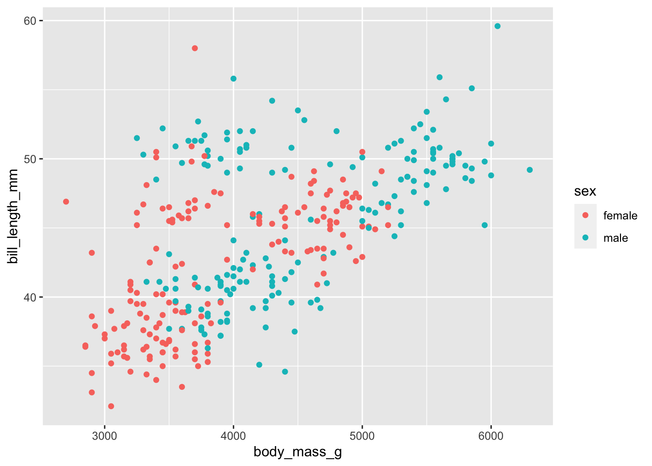

is equivalent to

penguins_complete <- penguins[complete.cases(penguins),]
penguins_complete |> 
  ggplot(aes(x = body_mass_g,y = bill_length_mm, color = sex)) +
geom_point()

Assignment 1

Load a data set referenced in Chapter 1 and create some kind of plot from it. See https://jonpage.github.io/r-course/intro.html for inspiration. Note the syntax to refer to a specific variable penguins$bill_length_mm.
Export the plot as an image and upload to your Samba Share folder.

.