Polynomial Data Fitting & Trigonometric Functions
Given a set of points sampled form a trig function in R^2, find the polynomial that contains them.
Contents
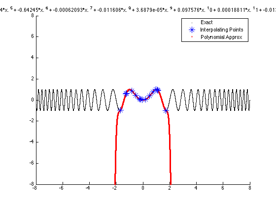
We choose random points on the graph of  .
.
	x_given = -2+4*rand(1,15);
    y_given = sin ((pi*x_given.^2 )/2);
	%y_given = exp(x_given.^2);

	n = length(x_given);
The "Coefficient" Matrix
The polynomial is a_0 + a_1*x + ... + a_m*x^m where m = n-1; This general form determines one equation for every given pair
	M = ones(n,n+1);
	for point = 1:n
		for i = 1:n;
			M(point,i) = x_given(point)^(i-1);
		end
		M(point,n+1) = y_given(point);
	end
Solve the system
	A = rref(M);
	a = A(:,end);
The polynomial
For example, y = a(1) + a(2)*x + a(3)*x.^2;
	r = 8; % How wide is the range of the plotting window
	x = -r:.0001:r; % a sample of x values in the chosen range
	s = [num2str(a(1))]; % make a string out of the number held in a(1)

	% term by term, make a polynomial whose coeffs are taken from a
	for i = 2:length(a);
	 	% s is a character string that looks like the poly we want
		s = [s,' + ',num2str(a(i)),'*x.^',num2str(i-1)];
	end
	% now we turn the character string into a set of y-values of the polynomial
	y = eval(s);
Plot the points and the curve in a psudo-animation
	close all; % close all other figures
	figure; % create a new figure
	ylim([-r r]); % the max/min of the y-axis
	xlim([-r r]); % the max/min of the x-axis
	hold on % put all the plots onto the same figure
	title(s); % puts the string s into the title

	xx = [-r:.001:r]; % sample x-values, the domain of the function
	yy = sin((pi*xx.^2)/2); % the exact function
	%yy = exp(xx.^2);
	plot(xx,yy,'sk','MarkerSize',1) % plot the exact function in black
	legend('Exact') % create a legend
	pause % pause the printing for greater appreciation

	% Plot the given points as large blue stars,
	plot(x_given,y_given,'*b','MarkerSize',12);
	legend('Exact', 'Interpolating Points')
	pause

	% Plot the graph of the polynomial along with the given points
	plot(x,y,'or','MarkerSize',2);
	plot(x_given,y_given,'*b','MarkerSize',12);
	legend('Exact','Interpolating Points', 'Polynomial Approx')