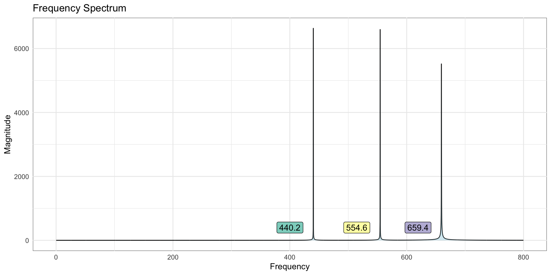
# librarieslibrary(seewave)library(stats) # create a waveform sample_rate =8000 k =5 a <-sin(2*pi*440.00*seq(0,k,length.out=sample_rate*k)) cs <-sin(2*pi*554.37*seq(0,k,length.out=sample_rate*k)) e <-sin(2*pi*659.25*seq(0,k,length.out=sample_rate*k)) s =1/3*(a+cs+e); # a pure "A" chord# function that performs the fft, and computes the modulus my_fft <-function(s){ f <-fft(s) m <-sqrt(Re(f)^2+Im(f)^2); df <-tibble(freq = f, m = m)return(df) }# apply fft to signal s df <-my_fft(s) df <-mutate(df, f =row_number() / k, og_sig = s, yl =400) |>relocate(f,.before =1) |>relocate(og_sig, .after =1)# plot zoomed in version of the full symmetric signal dl <-filter(df,f <800) |>arrange(-m) |>slice_head(n=3) df |>filter(f <800) |>ggplot(aes(x = f, y = m)) +geom_line() +geom_label(data = dl, aes(x = f, y = yl,label = f, fill =as_factor(f)), nudge_x =-40) +geom_ribbon(aes(ymin =0, ymax = m), fill ="lightblue", alpha =0.5) +labs(title ="Frequency Spectrum", x ="Frequency", y ="Magnitude") +theme_minimal() +theme(panel.background =element_rect(fill ="white", colour ="grey50"), legend.position ="none") +scale_fill_brewer(palette ="Set3")
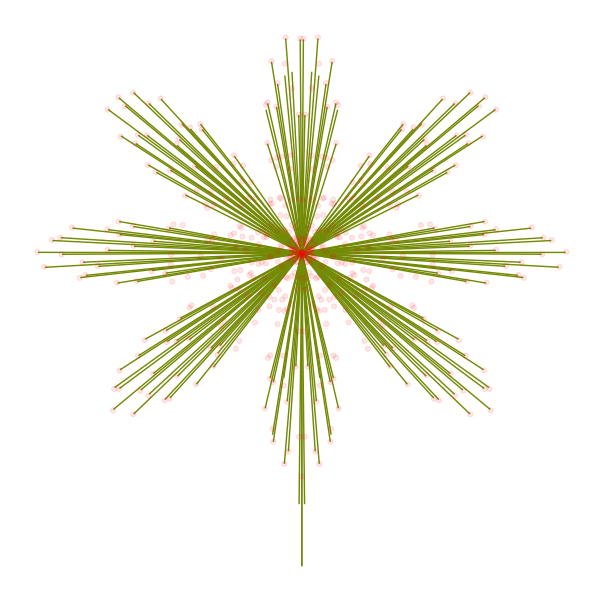
The parametric curve defined by \[f(t) = (\cos(44*2\pi t) + \cos(54*2\pi t))*\cos(2*\pi t) + i[ (\cos(44*2\pi t) + \cos(54*2\pi t))*\sin(2*\pi t)]\] is quite lovely but too complex to currently animate the Fourier series.
As consolation we display some Fourier vectors with relatively large magnitudes.
Animation was made in R using (roughly) the code below:
Code
library(av)library(ggforce)library(tidyverse)library(gganimate)# - - - D e f i n e C o n s t a n t s - - - ## K governs the time steps, i.e., sample the unit time interval @ 50 spots K =1000# t = seq(0,2*pi,length.out = K) # time, fed into f below u =seq(0,1,length.out=K) N =5# N sum from -N to N . # of circles 2N + 1 del =1/K # for approx. integration i <-complex(real =0, imaginary =1)f <-function(t){# -- -- -- S I M P L E S I N U S O I D -- -- -- ## f <- sin(2*pi*t)# O V A L -- -- -- -- -- -- ## the oval is *roughly* approximated when N = 10% of K# f <- complex(real = (1-tan(2*pi*t))*cos(2*pi*t), imaginary = sin(2*pi*t))# 3 L E A F C L O V E R -- -- -- -- -- # # also, ball-parked with N = 10% of K# f <- complex(real = cos(2*pi*t) + cos(4*pi*t) , imaginary = sin(2*pi*t) - sin(4*pi*t))# SIDEWAYS S, NOT PERIODIC# f <- complex(real = cos(2*pi*t) * cos(4*pi*t) , imaginary = sin(2*pi*t) * sin(4*pi*t))# - - - - - O.G. D U M B B E L L - - - - - - - - - # f <-complex(real =cos(2*pi*t) , imaginary =sin(3*sin(2*pi*t)))# O U T & B A C K C U R V E# f <- complex(real = 4*t*(1-t), imaginary = 0)# - - S A W T O O T H wave, i.e., drawing an O P E N horizontal line in C # f <- complex(real = t, imaginary = 0)# -- -- -- S Q U A R E W A V E -- -- -- -- ## f <- complex(real = t, imaginary = if_else(t <= 0, -1, 1))# REAL VALUED SQUARE WAVE# f <- complex(real = t, imaginary = sign(sin(2*pi * t)))# f <- sign(sin(2*pi * t))# # an A-minor chord / makes pretty flower# w = 2*pi# k = 500 AA =round(440/k) AA =44 CC =round(523.25/k) CC =52 EE =round(659.30/k) tt = t #f <- complex(real = (cos(w*AA*tt) + cos(w*CC*tt) + cos(w*EE*tt)) * cos(w*tt), # imaginary = (cos(w*AA*tt) + cos(w*CC*tt) + cos(w*EE*tt)) * sin(w*tt))#f <- complex(real = (cos(w*AA*tt) + cos(w*CC*tt)) * cos(w*tt), # imaginary = (cos(w*AA*tt) + cos(w*CC*tt)) * sin(w*tt))# a complicated loop#f <- complex(real = sin(10*pi*t) + 0.5*sin(20*pi*t)*cos(2*pi*t), # imaginary = sin(10*pi*t) + 0.5*sin(20*pi*t)*sin(2*pi*t))return(f)}# define f via data#f <- function(t){# wp = wonky_path(t,K)# return(wp$z[t])#}# fourier coeffs # why do we not divide by anything like we see in the real-valued definition?cn <-function(n,f,u,del){#1/(u[length(u)] - u[1])*sum(f(u)*exp(-n*2*pi*i*u)*del)sum(f(u)*exp(-n*2*pi*i*u)*del)}# ------- compute fourier coeffs ------- # c_n <-map(-N:N, ~cn(.,f,u,del)) |>unlist() # A returns the summands G =array()j =1# A <-function(t){for (n inc(-N:N)){ G[j] <- c_n[[j]] *exp(n*2*pi*i*t) j = j+1 }return(G)}# compute the series B =map(u,~sum(A(.))) |>unlist()# uncomment belowmytheme <-theme_minimal() +theme(panel.background =element_rect(fill ="white", colour ="grey50"), legend.position ="none")p <-ggplot() +# below is the ACTUAL map#geom_point(data=tibble(x=Re(f(u)),y=Im(f(u))), geom_point(data=tibble(x=u,y=f(u)), mapping =aes(x=x,y=y), color ="#859900", size =2, shape =1) +# Below is the fourier series (approximation)#geom_point(data=tibble(x=Re(B),y=Im(B)), geom_path(data=tibble(x=u,y=Re(B)), mapping =aes(x=x,y=y), color ="#6c71c4", size=1) + mytheme +labs(title="Sine Wave Fourier Approximation")# ggsave("~/googledrive/Research/Audio/sine-wave.png",p)# plot(Re(B),Im(B))
Code
library(av)library(ggforce)library(tidyverse)library(gganimate)library(vctrs)# these lines make sense after running fp3.R# fc$c is fourier coefficients# fc$n is the corresponding n# fourier coefs#C = fc$cix =-N:N#ix = fc$nz =which(ix ==0)# a =atan2(Im(C),Re(C))R =sqrt(Re(C)^2+Im(C)^2)# A has fourier coeffs, indexA =tibble(c = C,# n = ix,a = a,r = R)A <- A |>arrange(-desc(-n)) |>arrange(-desc(abs(n)))t =seq(0,1,length.out = K) # time# the summand of a fourier series# pass n in as c(-N:N)fn <-function(n,t){sum( C[which(ix %in% n)] *exp(2*pi*n*i*t))}# the value of the f-series when n = 0 and t = 1 firstn =floor(length(ix)/2)# the complex #, (vector) of the f-series at n-summands @ t fn_n <-function(n,t) {if (n >0) { jx = ix[ (z - n):(z + n) ] jx = jx[2:length(jx)]fn(jx,t) } else {fn(sort( ix[(z - n):(z + n)] ),t)} }# evaluate the series at the shown "n" s <-array(dim =c(length(t), firstn *2+1 ))# -- -- -- The Partial Sums of the Main Series -- -- -- -- I <-tibble(ix_seq = firstn:-firstn)ix_seq <- I |>arrange(-desc(abs(ix_seq))) |>pull()j =1for (n in ix_seq){ s[,j] <-map(t,~fn_n(n,.)) |>unlist() j = j+1}# -- -- -- The Partial Sums of the Main Series P I V O T E D -- -- -- #ss <-tibble(t = t, T =1:K, z_1 = s[,1]) for (r in2:dim(s)[2]){ name =str_c("z_",as.character(r)) ss <-mutate(ss, {{name}} := s[,r])}# Alternate way to pivot that maybe saves memory# <- select(ss,-1) |> # reshape2::melt(value.name = 'z', id = 'T') |># tibble()# Main data frame, used to produce all figures d <-tibble()for (n inc(1:dim(ss)[1])){# at the n-th moment in time the circles have the data below b <- ss |>slice(n) |>pivot_longer(-c(t,T),names_to =c(".value","n"),names_sep ="_") d <-bind_rows(b,d) } d <-mutate(d, n =as.numeric(n), r = A$r[n], znx = z[c(2:length(d$z),1)]) |>relocate(r, .after = znx)# half the vectors rotate in the opposite direction, color differently dpos <-filter(d, n != (2*N+1) & (n %%2==1)) dneg <-filter(d, n != (2*N+1) & (n %%2==0))# - - - N E E D E D T O H A C K R E V E A L - - - ## # the best approx. data (full series) dmax <-filter(d,n ==max(n)) ud <- u[1:length(u)-1] dtrue <-tibble(x=Re(f(ud)),y=Im(f(ud)))# - - - - P L O T B E G I N N I N G - - - - #p <-ggplot() +# sanity check geom: should give static path of the some unafilliated values# I Can CONFIRM that the # of elements in the 'new data' affects # the static / dynamic nature# geom_point(data=tibble(u=1:9,v=1:9),mapping=aes(x=u,y=v)) + # static plot of the true valuesgeom_point(data = dtrue, mapping =aes(x=x,y=y), color ="black",size=4, alpha = .1) +# want to plot a path connecting best-fit (top-level) or even true values#geom_path(data = dtrue, mapping = aes(x=u,y=w)) + #geom_point(data = d, mapping = aes(x=Re(z),y=Im(z)), color = "black", size=2) + # should be true values dynamic# geom_path(data = tibble(x=u, y=f(u), T=1:K),aes(x=Re(y),y=Im(y)), color = "red",size=8, alpha = 1) +# below: dot is a partial sum at the given moment in time#geom_path(d,mapping = aes(x=Re(z),y=Im(z)), color = "red",size=8, alpha = 0.1) +# best approx via partial fourier sums# different data => static plots IF the different data has no T# geom_point(data = tibble(x=Re(s[,dim(s)[2]]),# y=Im(s[,dim(s)[2]])),# aes(x=x,y=y), color = "blue",size = 8, alpha = 5) +# ----- REVEAL ------- approxiimation but it prints all the partial sums# geom_point(data = slice_head(dmax), # aes(x=Re(z),y=Im(z)), color = "black",size = 2, alpha = 1) +# another way to plot best approx (last_col of d), but make it dynamicgeom_point(data = dmax,aes(x=Re(z),y=Im(z)), color ="green",size =8, alpha =5) +geom_point(data = dmax,aes(x=Re(z),y=Im(z)), color ="black",shape =1, size =8) +## - - - - - - C I R C L E S & S E G M E N T S - - - - - - - ## # the origin & fixed vectorgeom_point(data =tibble(x=0,y=0), aes(x=x,y=x), color ="grey", size=5) +#geom_segment(data = d, aes(x = 0*Re(z[1]), y = 0*Im(z[1]), xend = Re(z[1]), yend = Im(z[1])), arrow = arrow(type = "closed", length = unit(0.30,"cm")), color = "#6c71c4") +# Add vectors - positivemap(1:nrow(dpos), ~geom_segment(data = dpos[.,],aes(x =Re(z), y =Im(z), xend =Re(znx), yend =Im(znx)),arrow =arrow(type ="closed", length =unit(0.10,"cm")), linewidth =2, color ="#859900")) +# Add vectors - negativemap(1:nrow(dneg), ~geom_segment(data = dneg[.,],aes(x =Re(z), y =Im(z), xend =Re(znx), yend =Im(znx)),arrow =arrow(type ="closed", length =unit(0.10,"cm")), linewidth =2, color ="#6c71c4")) +# Add C I R C L E Smap(1:nrow(d), ~geom_circle(data = d[., ],aes(x0 =Re(z), y0 =Im(z), r = r), color ="grey80", alpha =0.005)) +theme_void() +coord_fixed() +transition_states(T)animate(p, fps =10)anim_save("fourier-p.gif",animation =last_animation(),wd)#
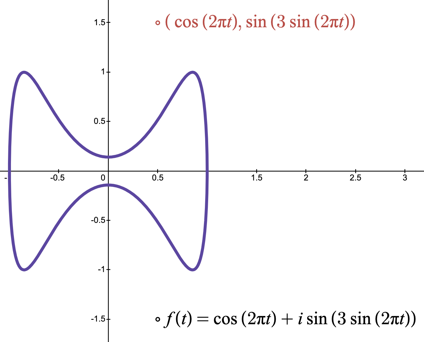
Fourier approximation of \(f(t) = \cos(2\pi t) + i \sin(3 \sin(2\pi t))\)
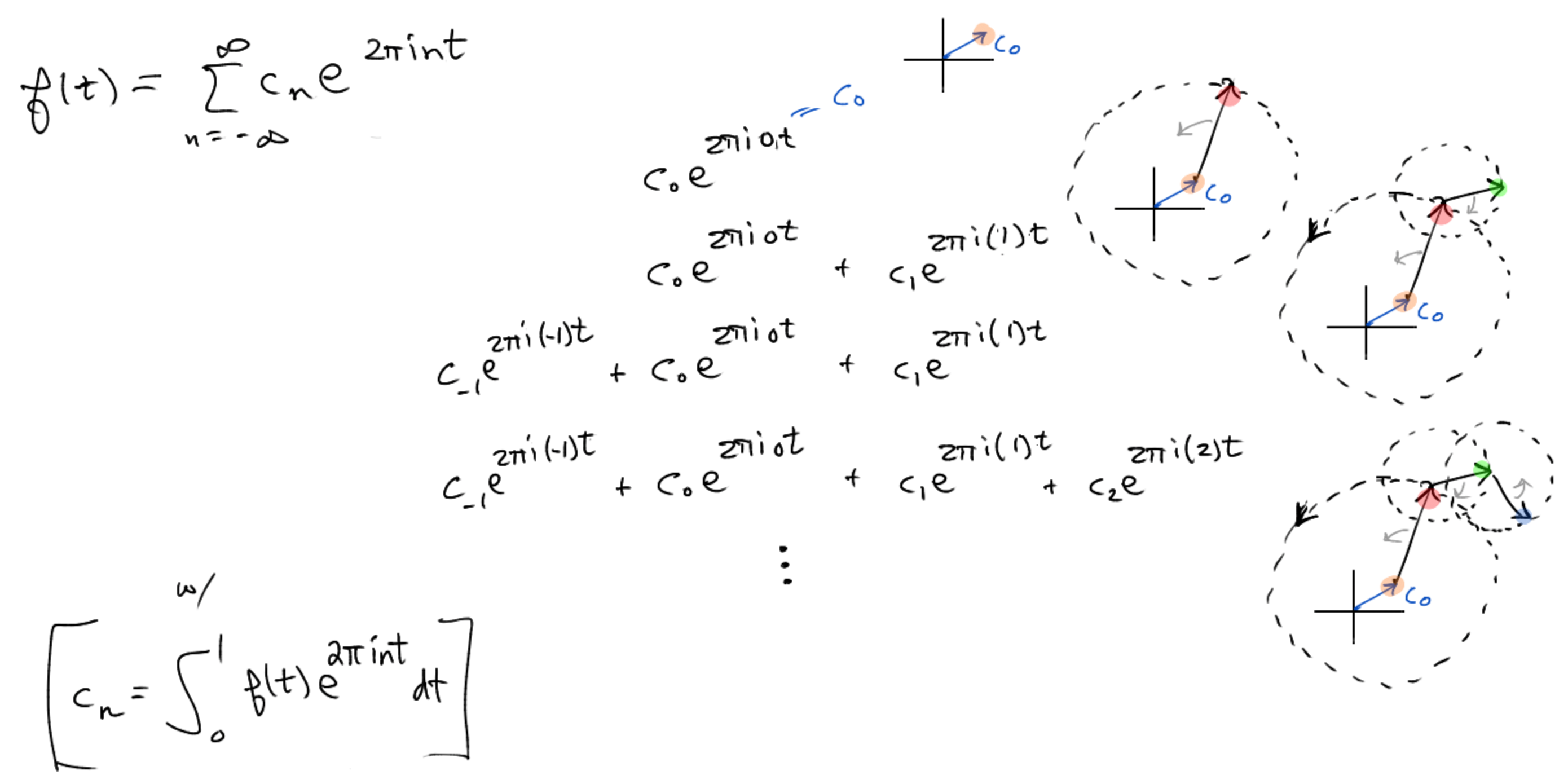
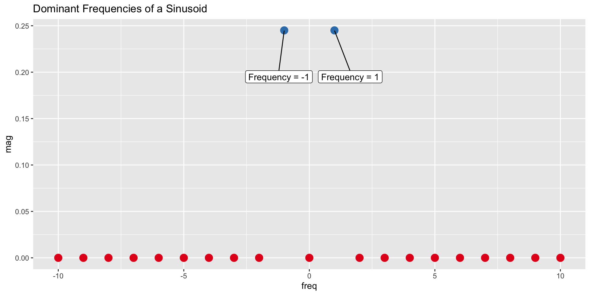
Recall, a Fourier series for \(\sin(t)\) is one where \[
\sin(t) = \sum_{k = -\infty}^{\infty} c_ke^{2 \pi i k t}
\] By Euler’s Identity \[
\begin{align*}
\sin(2\pi t) = \tfrac{1}{2i}e^{2 \pi i t} - \tfrac{1}{2i}e^{-2 \pi i t} \\
\end{align*}
\] So only two terms are necessary, i.e., \[
c_1 = \frac{1}{2i} \mbox{ and } c_2 = \frac{-1}{2i}
\]
The key property is the orthogonality of harmonically related exponentials: \[
\int_{0}^{1} e^{2 \pi i k t} e^{-2 \pi i n t} \mbox{d}t =
\begin{cases}
1 \mbox{ if } n = k\\
0 \mbox{ if } n \neq k
\end{cases}
\] Assuming the series for a signal \(s(t)\) converges \[
s(t) = \sum_{k = -\infty}^{\infty} c_ke^{2 \pi i k t}
\] Multiply both sides by \(e^{-2 \pi i n t}\) and integrate: \[
\int_0^1 s(t) e^{-2 \pi i n t} \mbox{d}t =
\int_0^1 \left(\sum_{k = -\infty}^{\infty} c_ke^{2 \pi i k t} e^{-2 \pi i n t} \mbox{d}t \right) =
\sum_{k = -\infty}^{\infty} \left(\int_0^1 c_ke^{2 \pi i k t} e^{-2 \pi i n t} \mbox{d}t \right) = c_k
\]
# - - - D e f i n e C o n s t a n t s - - - # K =100; # K governs the time steps, u =seq(0,1,length.out=K); # sampled time N =10# N is the number of terms in series del =1/K # for approx. integration i <-complex(real =0, imaginary =1)# -- -- -- S I M P L E S I N U S O I D -- -- -- # f <-function(t){ sin(2*pi*t) }# -- F O U R I E R C O E F F I C I E N T S -- # cn <-function(n,f,u,del){# approximate integration step for a fixed nsum( f(u) *exp(-n*2*pi*i*u)*del) }# get coeff for every n c_n <-map(-N:N, ~cn(.,f,u,del)) |>unlist()
The square wave is just the step function \[
\mbox{sq}(t) = \begin{cases}
1 \hskip{0.2 cm} \mbox{ if } 0 \leq x < 0.5 \\
-1 \hskip{0.2 cm}\mbox{ if } 0.5 < x <= 1 \end{cases}
\] The Fourier coefficients: \[
c_k = \int_0^{0.5} e^{-2 \pi i k t} \mbox{d}t - \int_{0.5}^{1} e^{-2 \pi i k t} \mbox{d}t
\] The u-substitution \(u = -2 \pi i k t\) gives \[
c_k = \tfrac{1}{-2 \pi i k t} \left( \int_0^{-\pi i k} e^{u} \mbox{d}u - \int_{-\pi i k}^{-2 \pi i k} e^{u} \mbox{d}u \right) = \tfrac{1}{-2 \pi i k t} (e^{-\pi i k} - 1 - e^{-2 \pi i k} + e^{-\pi i k})
\] Then manipulating exponents
\[
c_k = \tfrac{1}{-2 \pi i k t} \left((e^{-\pi i})^k - 1 - (e^{-2 \pi i})^k + (e^{-\pi i})^k)\right)
\] Which ultimately leads to \[
c_k = \tfrac{1}{-2 \pi i k t}(2(-1)^k -2) =
\begin{cases}
\frac{2}{\pi i k t} & \mbox{ if k odd} \\
0 & \mbox{ if k even}
\end{cases}
\]
The Fourier series for the square wave just uses odd multiples of the base frequency: \[
\mbox{sq}(t) = \sum_{k \in \{\dots -5,-3,-1,1,3,5 \dots\}} \frac{2}{\pi i k} e^{2 \pi i k t}
\]
And Euler’s Identity helps to see that this does indeed give a real number. Note that the sum includes both \(k\) and \(-k\). For example \[
\frac{2}{\pi i (-k) } e^{2 \pi i (-k) t} + \frac{2}{\pi i k } e^{2 \pi i k t} =
\frac{2}{\pi i (-k) } (\cos(2 \pi i (-k) t) + i\sin(2\pi i(-k)t)) +
\frac{2}{\pi i (k) } (\cos(2 \pi i (k) t) + i\sin(2\pi i(k)t))
\] The even / odd properties then lead to:
\[
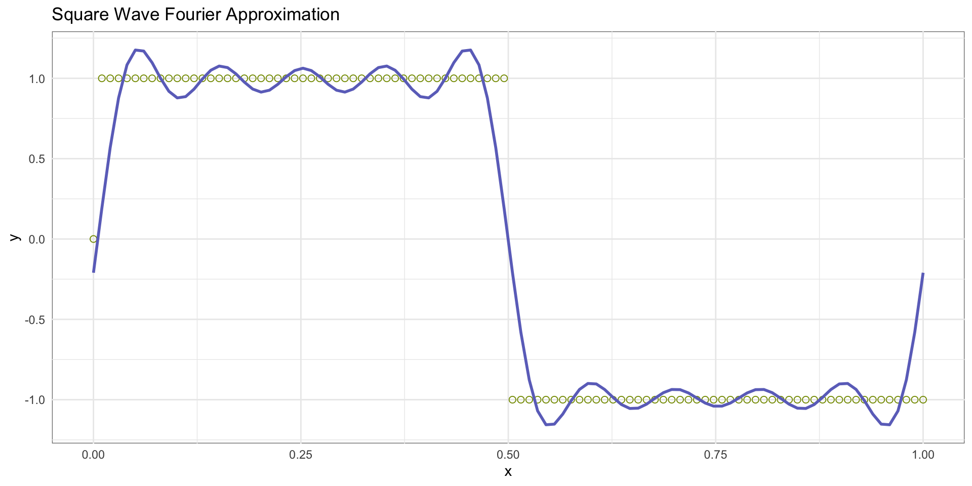
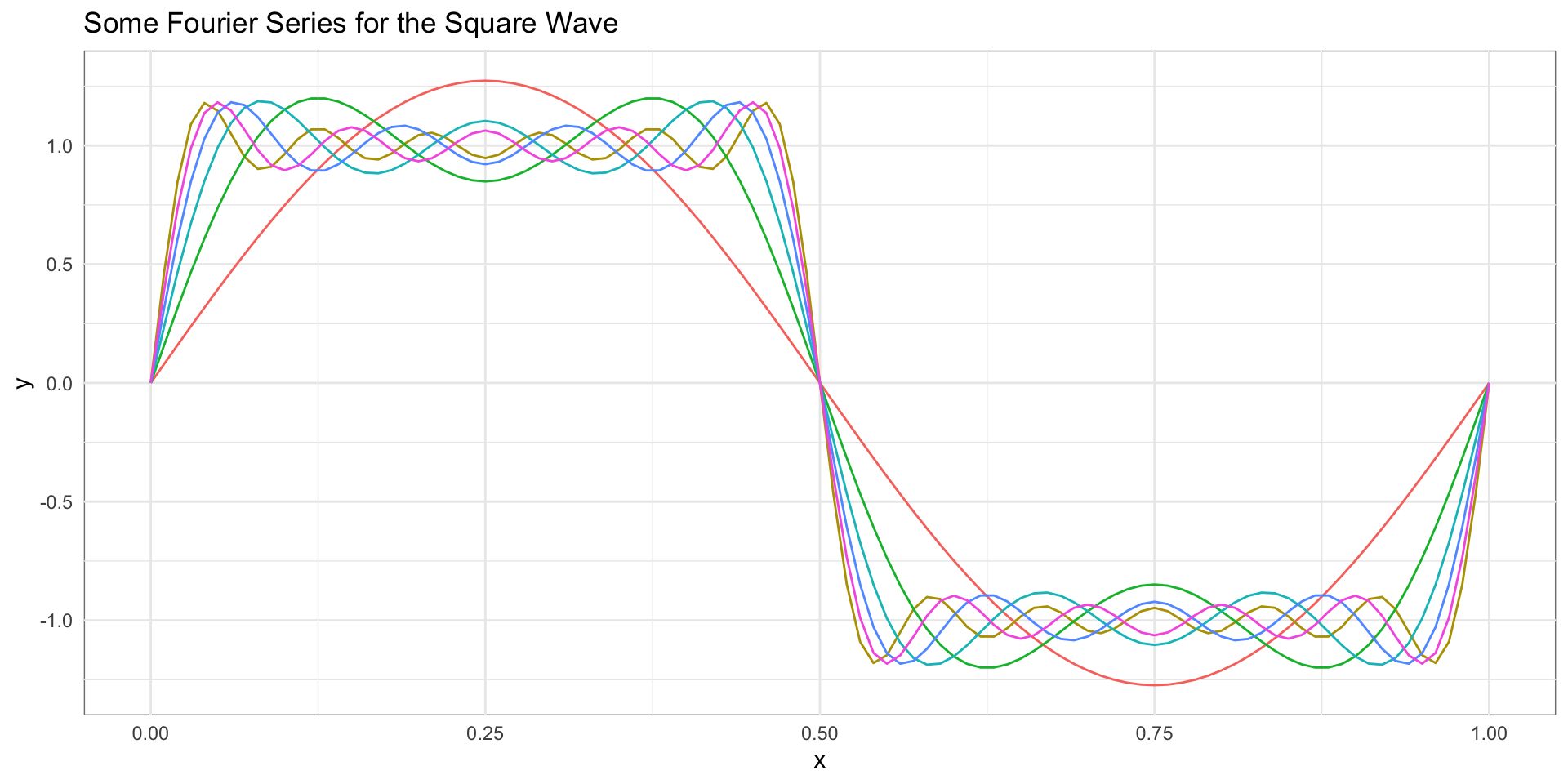
\mbox{sq}(t) = \sum_{k \in \{\dots,-5,-3,-1,1,3,5, \dots\}} \frac{2}{\pi k } \sin(2\pi k t) =
\sum_{k \in \{1,3,5, \dots\}} \frac{4}{\pi k } \sin(2\pi k t)
\]
Code
a =0; j =1;ff <-function(t,n){for (k inseq(1,n,2)) { a = a +4/(pi*k)*sin(2*pi*k*t)}return(a) }uu =seq(0,1,0.01)df <-tibble(x=uu, y_1=ff(uu,1), y_3=ff(uu,3), y_5=ff(uu,5), y_7=ff(uu,7), y_9=ff(uu,9), y_11=ff(uu,11)) |>pivot_longer(-x,values_to ="y", names_to ="name")ggplot(df,aes(x=x,y=y,group = name, color = name)) +geom_path() + mytheme +labs(title="Some Fourier Series for the Square Wave")