Voronoi Diagrams in R

library(devtools) # to install ggvoronoi
library(ggvoronoi) # easy voronoi plotting with ggplot
library(palmerpenguins)
library(sf) # spatial data analysis tools helpful for voronoi
library(tidyverse)

Description of Voronoi Diagrams

A Voronoi diagram is a way of dividing space into regions based on distance to a specific set of points. Each region contains all the points that are closer to one particular point than to any other. These diagrams are useful in various fields such as geography, meteorology, and computer science for tasks like spatial analysis and resource allocation.

Install ggvoronoi from github as

It was removed from cran for some reason. You will need to install devtools first if you don’t have it.

# install.packages("devtools") # run this line if you don't have devtools installed
install_github("garretrc/ggvoronoi")

Subset penguins data

d <- select(penguins, starts_with("bill"), species) |> 
  drop_na() |>
  rename(x = bill_depth_mm, y = bill_length_mm) |> 
  distinct() 

first voronoi diagram

ggplot(d, aes(x,y)) +
  stat_voronoi(geom="path") + 
  geom_point(aes(color = species))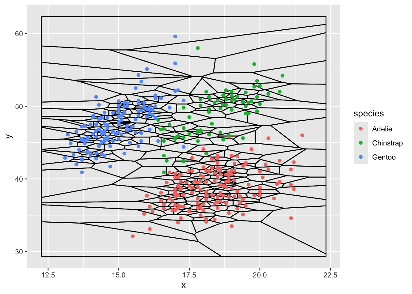

second voronoi diagram

ggplot(d) + geom_voronoi(aes(x,y,fill = species))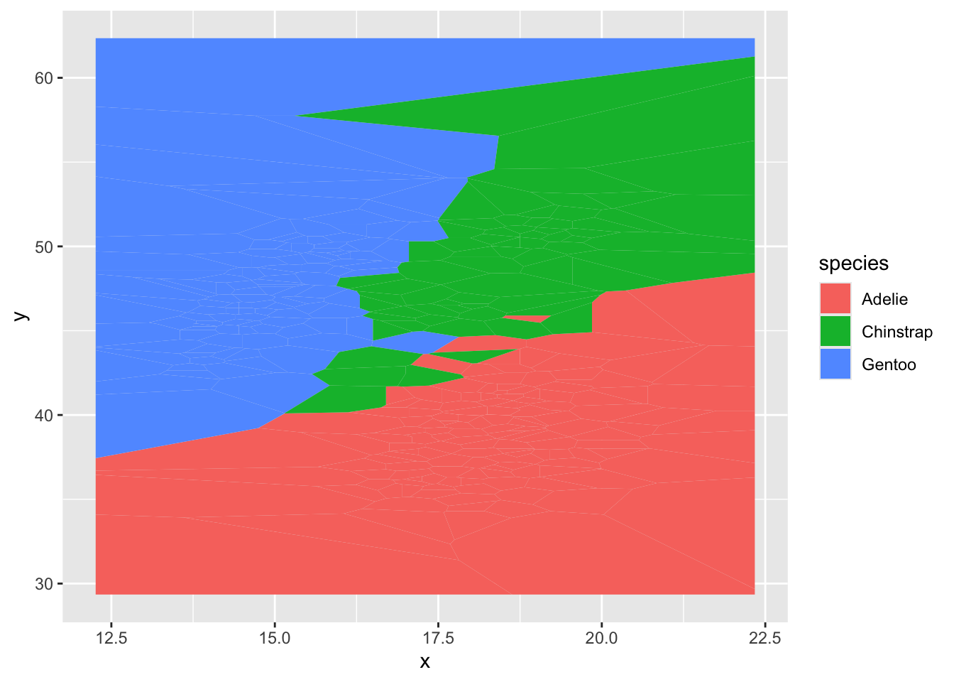

improve second

  ggplot(d) + geom_voronoi(aes(x,y,fill = species),color = "grey")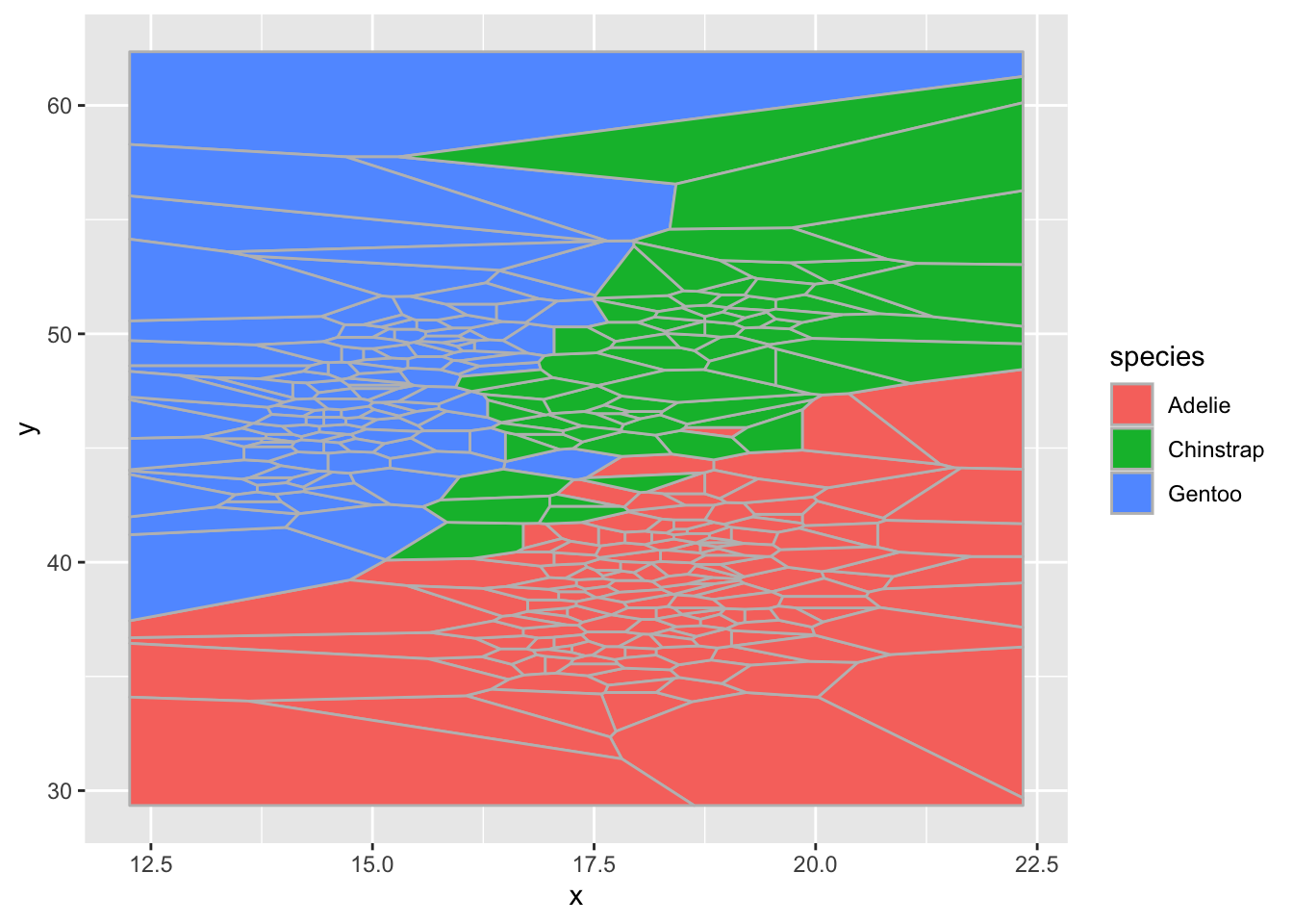

better second

  ggplot(d,aes(x,y)) + geom_voronoi(aes(fill = species),
                           color = "grey", alpha = .4) +
    geom_point(aes(color=species))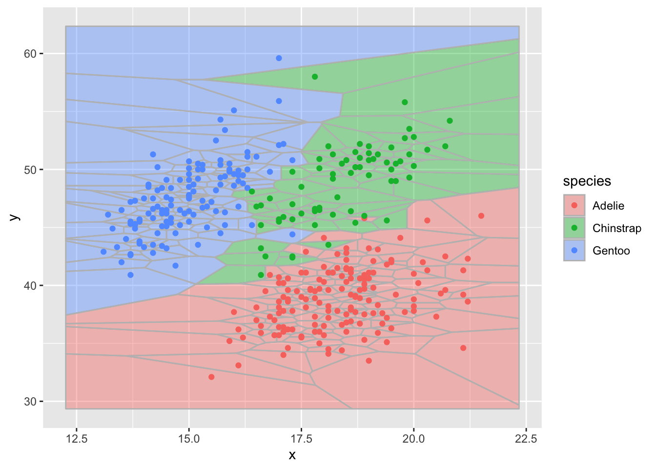 

Use geom_voronoi_tile to work compactify tiles

  ggplot(d,aes(x,y,group=-1L))  + 
  ggforce::geom_voronoi_tile(aes(fill = species), colour = 'black',
           alpha = .4, max.radius = 2) +   
    geom_point(aes(color=species))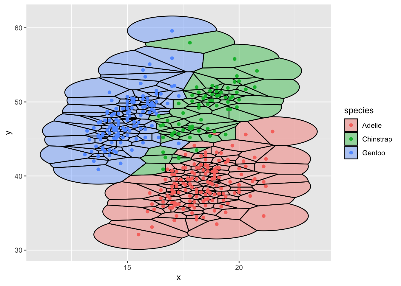 

# zoom as usual

  ggplot(d,aes(x,y,group=-1L))  + 
  ggforce::geom_voronoi_tile(aes(fill = species), colour = 'black',
           alpha = .4, max.radius = 2) +   
    geom_point(aes(color=species))  +
  scale_x_continuous(limits=c(16,20)) +
  scale_y_continuous(limits=c(40,50))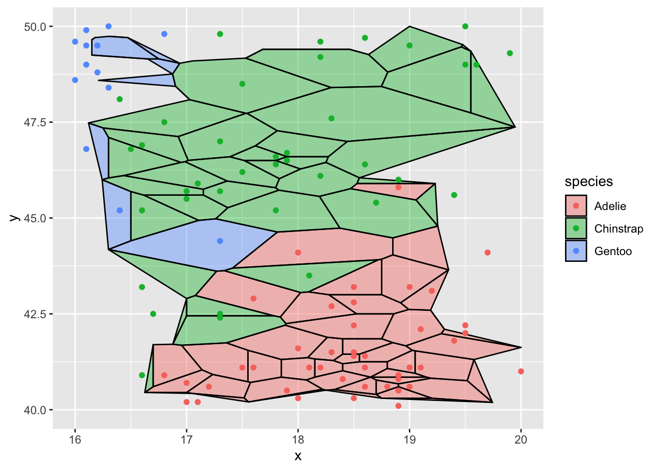 

M A K E - B O U N D I N G - C I R C L E

Plot a large circle around the data to improve the edges of the voronoi diagram

get the mean of the data

  mean_x <- mean(penguins$bill_depth_mm,na.rm=TRUE)
  mean_y <- mean(penguins$bill_length_mm,na.rm=TRUE)

range of data about mean

  d <- d |> mutate(dist2mean = sqrt((y-mean_y)^2+(x-mean_x)^2))

radius

rad <- max(d$dist2mean)
circle <- data.frame(x = mean_x+rad*cos(seq(0, 2*pi, length.out = 25)),
                     y = mean_y+rad*sin(seq(0, 2*pi, length.out = 25)),
                     group = rep(1,25))

another approach to improving the edges

ggplot(d,aes(x,y,group=-1L))  + 
  geom_voronoi(
    aes(fill = species), colour = 'black',alpha = .4, 
      outline = circle) +   
  geom_point(aes(color=species))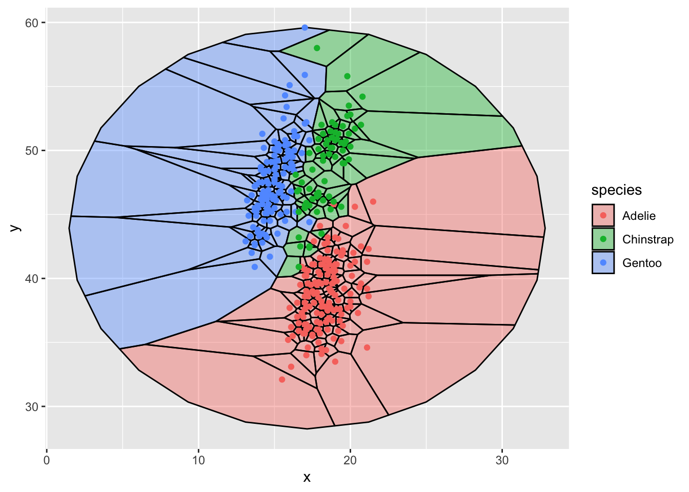 

first voronoi diagram with circle outline

ggplot(d, aes(x,y)) +
  stat_voronoi(geom="path", outline = circle) + 
  geom_point(aes(color = species))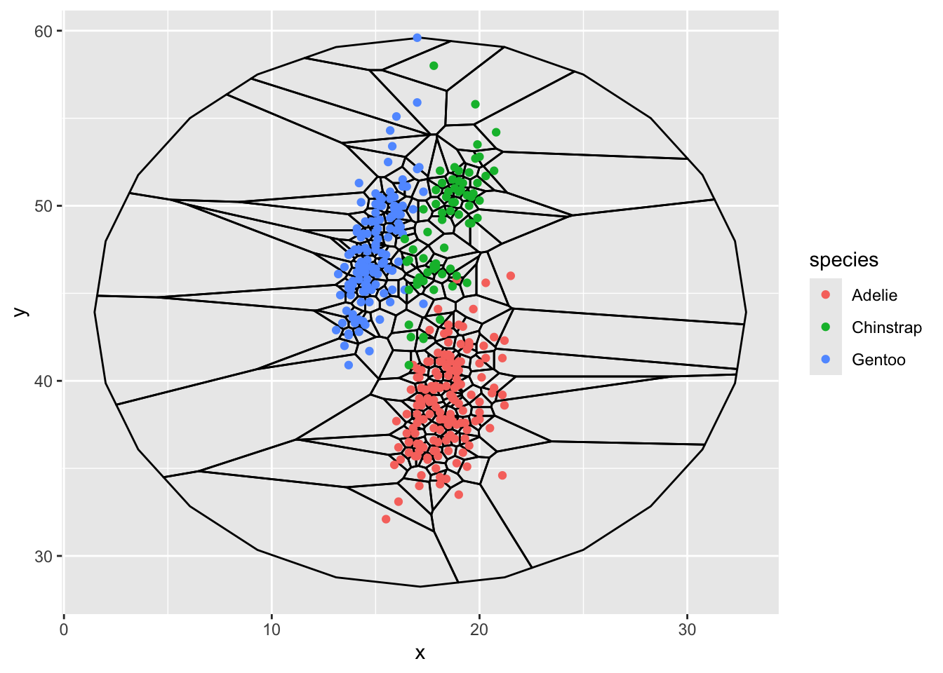

how could we use this to classify data

Suppose you find a new penguin with bill_depth = 15.3 and bill_length = 43.

What is the most likely species of this new penguin?

We can make a guess by looking at the graph.

  newp <- tibble(x=15.3,y=43) # a new point

  p <- ggplot(d, aes(x,y)) +
    geom_voronoi(aes(fill=species),
                 outline = circle, 
                 color = "grey")  +
    scale_fill_viridis_d(option = "D",alpha=.5) +
    geom_point(aes(color=species)) +
    scale_color_viridis_d(option = "H",alpha=.5) + 
    geom_point(data=newp,
               mapping = aes(x,y),
               shape = 7) +
    scale_x_continuous(limits=c(12,25)) +
    scale_y_continuous(limits=c(35,50)) 
  
  p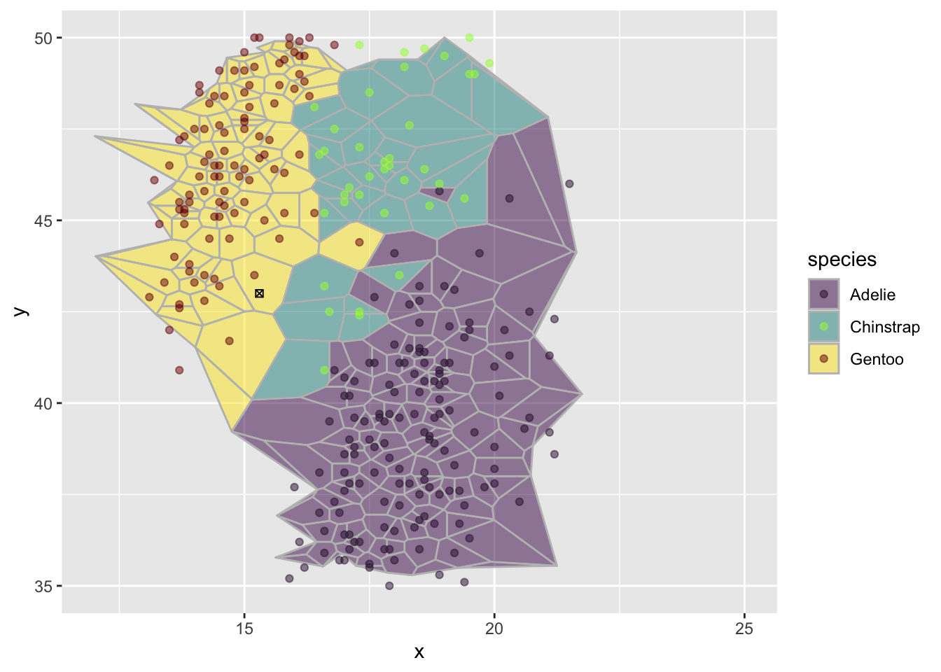

goal: compare new penguin to the centroid of each cell

create pts from raw data

Convert the x,y data into sf format

pts <- tibble(x = d$x, y = d$y, species = d$species) %>%
  st_as_sf(coords = c('x', 'y')) %>%
  st_set_crs(4326) 

turn circle data into sf format

cc <- select(circle,1:2) |> as.data.frame()
c_df <- st_as_sf(x = cc,coords = c("x", "y"), crs = "4326")

voronoi of pts

vor <- st_voronoi(st_combine(pts))

st_voronoi

st_voronoi returns a GEOMETRYCOLLECTION, and some plotting methods can’t use a GEOMETRYCOLLECTION.

this returns polygons instead

vor_poly <- st_collection_extract(vor)

to put a bounding box around the sf data

 box <- st_bbox(c_df) |> st_as_sfc()
 vcrop <- st_crop(vor_poly, box)
 plot(vcrop)

compute centroid of each cell

cntrd1 <- vor_poly |> st_centroid()

the coordinates of the centroid data

cntrd <- st_coordinates(cntrd1) |> as_tibble() |> 
  janitor::clean_names() |>
  mutate(centroid_x = x, centroid_y = y)

plot the centroids

p + geom_point(data=cntrd,aes(x,y),shape = 4) 

combine raw data and voronoi polygons

df <- cbind(pts,vor_poly) |> as_tibble() |> 
  rename(poly = geometry.1, point = geometry)

combine voronoi polygons, the raw data and centroids

a <- cbind(df, cntrd) |> tibble() |> rename(geometry=poly)

data containing the nearest centroid

nearest_cntrd <- mutate(cntrd,
                   d = sqrt((x-newp$x)^2 + (y-newp$y)^2)) |> 
                   arrange(d) |> slice_head()

the predicted species

filter(a,x==nearest_cntrd$x & y==nearest_cntrd$y) |> select(species)

# A tibble: 1 × 1
  species
  <fct>  
1 Adelie