library(tidyverse)
x <- c("1.2", "5.6", "1e3")
parse_double(x)
[1] 1.2 5.6 1000.0#> [1] 1.2 5.6 1000.0using dplyr
Standard techniques for working with numerical data in R using the dplyr package.
parse_doublelibrary(tidyverse)
x <- c("1.2", "5.6", "1e3")
parse_double(x)[1] 1.2 5.6 1000.0#> [1] 1.2 5.6 1000.0For numbers with formatting (like currency symbols, commas, or percentage signs), use parse_number():
x <- c("$1,234", "USD 3,513", "59%")
parse_number(x)
[1] 1234 3513 59#> [1] 1234 3513 59A (perhaps surprising) amount of data science can be done with simple tools like counts & summaries.
Often used with group_by(), count() is a convenient way to get the number of observations in each group.
count()# how many rows are in the diamonds dataset
count(diamonds)# A tibble: 1 × 1
n
<int>
1 53940# how many fair diamonds are there?
count(diamonds, cut = "Fair")# A tibble: 1 × 2
cut n
<chr> <int>
1 Fair 53940# note, the code above does not throw an error, but it does not do what you want. It's an example of something an AI might suggest that is incorrect. The correct code is below:
count(diamonds, cut)# A tibble: 5 × 2
cut n
<ord> <int>
1 Fair 1610
2 Good 4906
3 Very Good 12082
4 Premium 13791
5 Ideal 21551# or if you really ONLY wanted the "Fair" cut diamonds
count(diamonds, cut) |> filter(cut == "Fair")# A tibble: 1 × 2
cut n
<ord> <int>
1 Fair 1610To count unique values, or unique combinations dplyr provides n_distinct().
n_distinct()# how many unique cuts are there?
n_distinct(diamonds$cut)[1] 5# it's often used inside summarize()
# number of models per manufacturer
mpg |> group_by(manufacturer) |>
summarize(n_models = n_distinct(model)) |>
arrange(desc(n_models))# A tibble: 15 × 2
manufacturer n_models
<chr> <int>
1 toyota 6
2 chevrolet 4
3 dodge 4
4 ford 4
5 volkswagen 4
6 audi 3
7 nissan 3
8 hyundai 2
9 subaru 2
10 honda 1
11 jeep 1
12 land rover 1
13 lincoln 1
14 mercury 1
15 pontiac 1Below are some common ways to produce new numbers from existing ones.
R recycles vectors. It can be a useful feature, but can also lead to unexpected results. For example:
x <- seq(1,20,by = 2)
y <- c(1,2)

# explain x/yThe arithmetic functions work with pairs of variables. Two closely related functions are pmin() and pmax(), which when given two or more variables will return the smallest or largest value in each row:
df <- tribble(
  ~x, ~y,
  1,  3,
  5,  2,
  7, NA,
)

# notice the difference between min/max and pmin/pmax
df |>
  mutate(
    min = min(x, y, na.rm = TRUE),
    max = max(x, y, na.rm = TRUE),
    row_min = pmin(x, y, na.rm = TRUE),
    row_max = pmax(x, y, na.rm = TRUE)
  )
# A tibble: 3 × 6
x y min max row_min row_max
<dbl> <dbl> <dbl> <dbl> <dbl> <dbl>
1 1 3 1 7 1 3
2 5 2 1 7 2 5
3 7 NA 1 7 7 7Look at the format of dep_time. We can see that 517 means the time 5:17. Use modular arithmetic %% (the remainder after division) and integer division %/% (divide, but ignore remainder) to produce new variables of hour and minute.
Rows: 336,776
Columns: 19
$ year           <int> 2013, 2013, 2013, 2013, 2013, 2013, 2013, 2013, 2013, 2…
$ month          <int> 1, 1, 1, 1, 1, 1, 1, 1, 1, 1, 1, 1, 1, 1, 1, 1, 1, 1, 1…
$ day            <int> 1, 1, 1, 1, 1, 1, 1, 1, 1, 1, 1, 1, 1, 1, 1, 1, 1, 1, 1…
$ dep_time       <int> 517, 533, 542, 544, 554, 554, 555, 557, 557, 558, 558, …
$ sched_dep_time <int> 515, 529, 540, 545, 600, 558, 600, 600, 600, 600, 600, …
$ dep_delay      <dbl> 2, 4, 2, -1, -6, -4, -5, -3, -3, -2, -2, -2, -2, -2, -1…
$ arr_time       <int> 830, 850, 923, 1004, 812, 740, 913, 709, 838, 753, 849,…
$ sched_arr_time <int> 819, 830, 850, 1022, 837, 728, 854, 723, 846, 745, 851,…
$ arr_delay      <dbl> 11, 20, 33, -18, -25, 12, 19, -14, -8, 8, -2, -3, 7, -1…
$ carrier        <chr> "UA", "UA", "AA", "B6", "DL", "UA", "B6", "EV", "B6", "…
$ flight         <int> 1545, 1714, 1141, 725, 461, 1696, 507, 5708, 79, 301, 4…
$ tailnum        <chr> "N14228", "N24211", "N619AA", "N804JB", "N668DN", "N394…
$ origin         <chr> "EWR", "LGA", "JFK", "JFK", "LGA", "EWR", "EWR", "LGA",…
$ dest           <chr> "IAH", "IAH", "MIA", "BQN", "ATL", "ORD", "FLL", "IAD",…
$ air_time       <dbl> 227, 227, 160, 183, 116, 150, 158, 53, 140, 138, 149, 1…
$ distance       <dbl> 1400, 1416, 1089, 1576, 762, 719, 1065, 229, 944, 733, …
$ hour           <dbl> 5, 5, 5, 5, 6, 5, 6, 6, 6, 6, 6, 6, 6, 6, 6, 5, 6, 6, 6…
$ minute         <dbl> 15, 29, 40, 45, 0, 58, 0, 0, 0, 0, 0, 0, 0, 0, 0, 59, 0…
$ time_hour      <dttm> 2013-01-01 05:00:00, 2013-01-01 05:00:00, 2013-01-01 0…
# divide but drop remainder
hour <- flights$sched_dep_time %/% 100
# the remainder of 517 after dividing by 100 is 17
min <- flights$sched_dep_time %% 100Recall, to find the proportion of cancelled flights per month we can do:
flights |> group_by(month) |>
  summarize(prop_cancelled = mean(is.na(dep_time)))
# A tibble: 12 × 2
month prop_cancelled
<int> <dbl>
1 1 0.0193
2 2 0.0505
3 3 0.0299
4 4 0.0236
5 5 0.0196
6 6 0.0357
7 7 0.0319
8 8 0.0166
9 9 0.0164
10 10 0.00817
11 11 0.00854
12 12 0.0364 Use this idea with our new arithmetic tools to see how the proportion of cancelled flights varies throughout the day.
flights |>
  # create a variable hour from sched_dep_time and group by it.
  group_by(hour = sched_dep_time %/% 100) |>
  summarize(prop_cancelled = mean(is.na(dep_time)), n = n()) |>
  filter(hour > 1) |>
  ggplot(aes(x = hour, y = prop_cancelled)) +
  geom_line(color = "grey") +
  geom_point(aes(size = n)) +
  labs(title =
         "Proportion of Cancelled Flights Throughout the Day") +
  theme_minimal()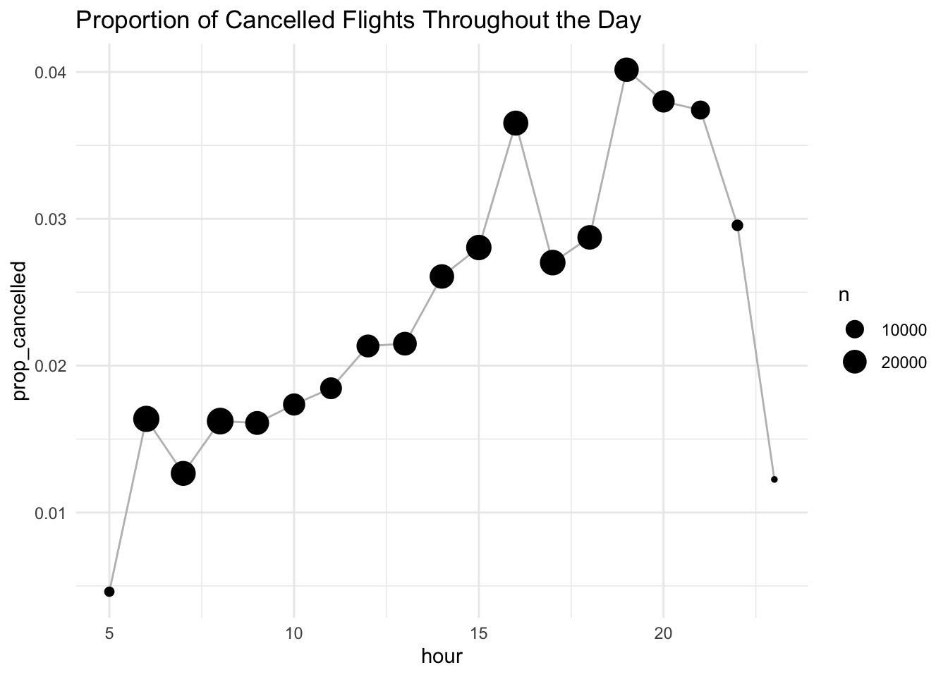
round() uses what’s known as “round half to even” or Banker’s rounding: if a number is half way between two integers, it will be rounded to the even integer. This is a good strategy because it keeps the rounding unbiased: half of all 0.5s are rounded up, and half are rounded down.
round(c(1.5, 2.5))[1] 2 2Here’s some common uses of rounding.
x <- 123.456
# Round down to nearest two digits
floor(x / 0.01) * 0.01
[1] 123.45# Round up to nearest two digits
ceiling(x / 0.01) * 0.01[1] 123.46# Round to nearest multiple of 4
round(x / 4) * 4[1] 124# Round to nearest 0.25
round(x / 0.25) * 0.25[1] 123.5Use cut() to break up (aka bin) a numeric vector into discrete buckets:
x <- c(1, 2, 5, 10, 15, 20)
cut(x, breaks = c(0, 5, 10, 15, 20))
[1] (0,5] (0,5] (0,5] (5,10] (10,15] (15,20]
Levels: (0,5] (5,10] (10,15] (15,20]The breaks don’t need to be evenly spaced:
cut(x, breaks = c(0, 5, 10, 100))[1] (0,5] (0,5] (0,5] (5,10] (10,100] (10,100]
Levels: (0,5] (5,10] (10,100]You can optionally supply your own labels. Note that there should be one less labels than breaks.
cut(x,
  breaks = c(0, 5, 10, 15, 20),
  labels = c("sm", "md", "lg", "xl")
)
[1] sm sm sm md lg xl
Levels: sm md lg xlExercise: Add a new variable to the diamonds data describing the price of each diamond.
Base R provides cumsum(), cumprod(), cummin(), cummax() for running, or cumulative, sums, products, mins and maxes. dplyr provides cummean() for cumulative means. Cumulative sums tend to come up the most in practice:
x <- 1:10
cumsum(x)
[1] 1 3 6 10 15 21 28 36 45 55#> [1] 1 3 6 10 15 21 28 36 45 55To assign a ranking use min_rank()
x <- c(10, 2, 12, 3, 4, NA)
min_rank(x)
[1] 4 1 5 2 3 NANote that the smallest values get the lowest ranks; use desc(x) to give the largest values the smallest ranks:
min_rank(desc(x))[1] 2 5 1 4 3 NArow_number() can also be used without any arguments when inside a dplyr verb. In this case, it’ll give the number of the “current” row. When combined with %% or %/% this can be a useful tool for dividing data into similarly sized groups:
df <- tibble(id = 1:10)

df |>
  mutate(
    row0 = row_number() - 1,
    three_groups = row0 %% 3,
    three_in_each_group = row0 %/% 3
  )
# A tibble: 10 × 4
id row0 three_groups three_in_each_group
<int> <dbl> <dbl> <dbl>
1 1 0 0 0
2 2 1 1 0
3 3 2 2 0
4 4 3 0 1
5 5 4 1 1
6 6 5 2 1
7 7 6 0 2
8 8 7 1 2
9 9 8 2 2
10 10 9 0 3Exercise: Use this idea to place randomly place everyone in this room into groups of 2.
Sometimes you want to start a new group every time some event occurs. For example, when you’re looking at website data, it’s common to want to break up events into sessions, where you begin a new session after gap of more than x minutes since the last activity. For example, imagine you have the times when someone visited a website:
events <- tibble(
  time = c(0, 1, 2, 3, 5, 10, 12, 15, 17, 19, 20, 27, 28, 30)
)
And you’ve computed the time between each event, and figured out if there’s a gap that’s big enough to qualify:
events <- events |>
  mutate(
    diff = time - lag(time, default = first(time)),
    has_gap = diff >= 5
  )
events
# A tibble: 14 × 3
time diff has_gap
<dbl> <dbl> <lgl>
1 0 0 FALSE
2 1 1 FALSE
3 2 1 FALSE
4 3 1 FALSE
5 5 2 FALSE
6 10 5 TRUE
7 12 2 FALSE
8 15 3 FALSE
9 17 2 FALSE
10 19 2 FALSE
11 20 1 FALSE
12 27 7 TRUE
13 28 1 FALSE
14 30 2 FALSE Use cumsum() to go from the boolean vector above to a numeric vector that you can group_by().
events |> mutate(
  group = cumsum(has_gap)
)
# A tibble: 14 × 4
time diff has_gap group
<dbl> <dbl> <lgl> <int>
1 0 0 FALSE 0
2 1 1 FALSE 0
3 2 1 FALSE 0
4 3 1 FALSE 0
5 5 2 FALSE 0
6 10 5 TRUE 1
7 12 2 FALSE 1
8 15 3 FALSE 1
9 17 2 FALSE 1
10 19 2 FALSE 1
11 20 1 FALSE 1
12 27 7 TRUE 2
13 28 1 FALSE 2
14 30 2 FALSE 2Now you can use group_by(group) to analyze each session separately.
events |>
  mutate(
    group = cumsum(has_gap)
  ) |>
  group_by(group) |>
  summarize(
    start = min(time),
    end = max(time),
    n_events = n()
  )
# A tibble: 3 × 4
group start end n_events
<int> <dbl> <dbl> <int>
1 0 0 5 5
2 1 10 20 6
3 2 27 30 3quantile() is a generalization of the median: quantile(x, 0.25) will find the value of x that is greater than 25% of the values, quantile(x, 0.5) is equivalent to the median, and quantile(x, 0.95) will find the value that’s greater than 95% of the values.
For the flights data, you might want to look at the 95% quantile of delays rather than the maximum, because it will ignore the 5% of most delayed flights which can be quite extreme.
flights |>
  group_by(year, month, day) |>
  summarize(
    max = max(dep_delay, na.rm = TRUE),
    q95 = quantile(dep_delay, 0.95, na.rm = TRUE),
    num_badly_delayed = sum(dep_delay > q95, na.rm = TRUE),
    .groups = "drop"
  )
# A tibble: 365 × 6
year month day max q95 num_badly_delayed
<int> <int> <int> <dbl> <dbl> <int>
1 2013 1 1 853 70.1 42
2 2013 1 2 379 85 45
3 2013 1 3 291 68 44
4 2013 1 4 288 60 43
5 2013 1 5 327 41 35
6 2013 1 6 202 51 41
7 2013 1 7 366 51.6 47
8 2013 1 8 188 35.3 45
9 2013 1 9 1301 27.2 45
10 2013 1 10 1126 31 46
# ℹ 355 more rowsx / sum(x) calculates the proportion of a total.
(x - mean(x)) / sd(x) computes a Z-score (standardized to mean 0 and sd 1).
(x - min(x)) / (max(x) - min(x)) standardizes to range [0, 1].
x / first(x) computes an index based on the first observation.
x / lag(x) computes period-over-period growth rates.
x / lead(x) computes period-over-period decay rates.
x / nth(x, n) computes an index based on the nth observation.