# get the working diretory
getwd()
# set the working directory
# note: Windows users, use forward slash \
setwd("enter your directory here")Exploring a real dataset
Exploratory Data Analysis
This set of exercises exposes you to several important aspects of data science.
- This is a big dataset (relatively speaking)
- It’s been touched by many hands, and the artifacts show.
- It involves download, import as well as installing tools specific for this dataset.
ATUS Data
Learn more and extract different data below: American Time Use Survey
Our ATUS data concerns sex, age, race, stress & work
Download
Download the codebook, the ddi file and the zip file. ddi codebook .zip
Prepare to download the data into your Dat309 folder (not Samba!), or a suitable sub-directory. Make sure RStudio can see your newly downloaded files. Click Session > Set Working Directory > Choose Directory
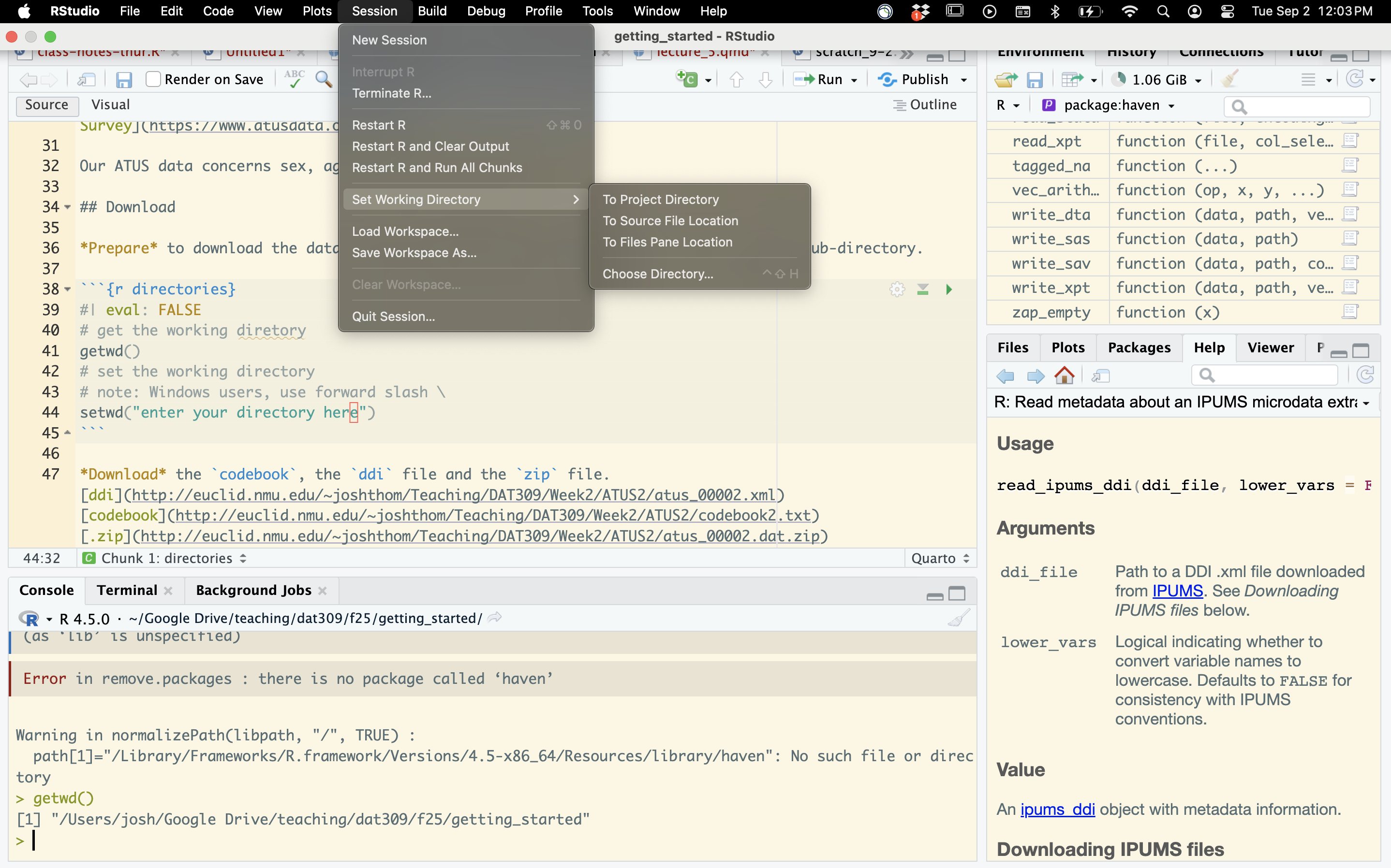
Or, do it by hand using these commands.
Use the codebook to parse meaning from the variables. You need the ipumsr package to load the data into R.
# haven contains functions that covert the data into an r-friendly format
install.packages("haven")
install.packages("ipumsr")
# load ATUS data
# The data requires the IPUMSr package
library(haven)
library(ipumsr)
ddi <- read_ipums_ddi("ATUS2/atus_00002.xml")
data <- read_ipums_micro(ddi)Use of data from IPUMS ATUS is subject to conditions including that users should cite the data appropriately. Use command `ipums_conditions()` for more details.detach("package:haven", unload=TRUE)Warning: 'haven' namespace cannot be unloaded:
namespace 'haven' is imported by 'ipumsr' so cannot be unloadedExploratory Questions
- What is the size of the data? How many rows & columns? (Use
dim(), for dimension.) - What do the numbers mean in the rows?
- What are the variable names and what do they mean?
The (very useful) clean_names() function makes the variable names a bit easier to read.
# filter to get stress data
#| eval: TRUE
library(tidyverse)
Warning: package 'purrr' was built under R version 4.5.1── Attaching core tidyverse packages ──────────────────────── tidyverse 2.0.0 ──
✔ dplyr 1.1.4 ✔ readr 2.1.5
✔ forcats 1.0.0 ✔ stringr 1.5.1
✔ ggplot2 3.5.2 ✔ tibble 3.3.0
✔ lubridate 1.9.4 ✔ tidyr 1.3.1
✔ purrr 1.1.0
── Conflicts ────────────────────────────────────────── tidyverse_conflicts() ──
✖ dplyr::filter() masks stats::filter()
✖ dplyr::lag() masks stats::lag()
ℹ Use the conflicted package (<http://conflicted.r-lib.org/>) to force all conflicts to become errorslibrary(janitor)
Attaching package: 'janitor'

The following objects are masked from 'package:stats':

    chisq.test, fisher.test
ds <- clean_names(data)
ds <- filter(ds,scstress < 10)The variable pertaining to “kind of job” was poorly named, so we change it.
# rename work variable
#| eval: FALSE
ds <- filter(ds,scstress < 10)
ds <- rename(ds,"job" = occ2_cps8)
Filter
Choose a few jobs so the data isn’t so big. Learn what how the numbers relate to jobs in the codebook.
dmsf <- filter(ds,job == 120 | job == 122 |job == 132)
ggplot(dmsf,aes(x=scstress)) + geom_bar()
Visualizing Distributions & Relationships
Categorical distribution: bar plot
Numerical distribution: histogram, density plot
Numerical distribution vs. categorical variable: box plot
Two categorical variables: barplot filled with color or the same with
position = "fill"in the geom.Two-Three numerical variables: scatter plot with colors mapped to a variable. (see text)
Just a few categorical variables? Try faceting:
Exercise 1. Improve the plot below with fill = as_factor(job) from the haven package.
2. Add a position = "fill" to the geom_bar(). Does it help?
dmsf <- filter(ds,job == 120 | job == 122 |job == 132)
ggplot(dmsf,aes(x=scstress, fill = job)) + geom_bar() +
  labs(fill = "Job")
Warning: The following aesthetics were dropped during statistical transformation: fill.
ℹ This can happen when ggplot fails to infer the correct grouping structure in
the data.
ℹ Did you forget to specify a `group` aesthetic or to convert a numerical
variable into a factor?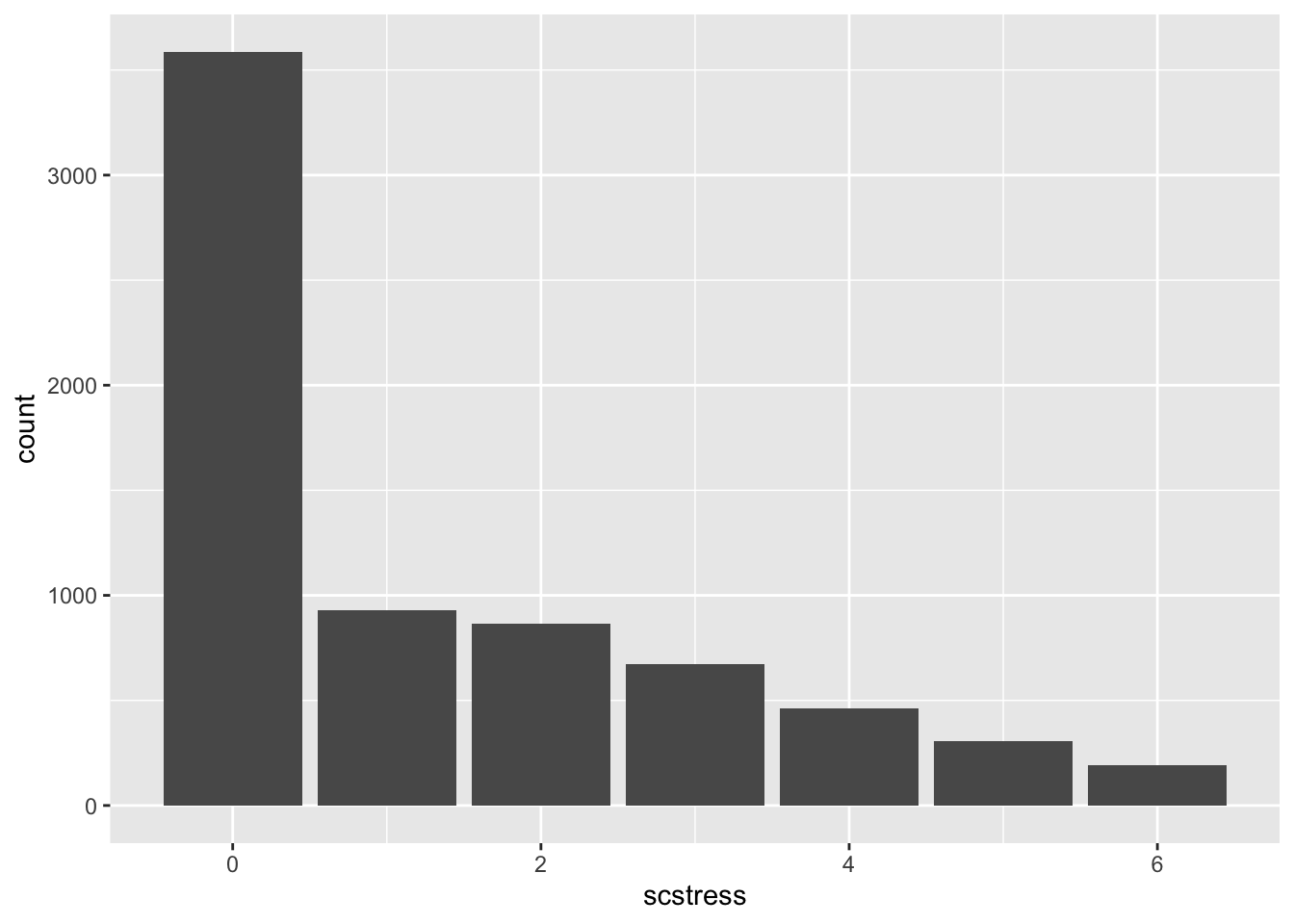
Factors
- Remove
factor()from thefill = factor(job)and observe the result. - Replace it with
fill = haven::as_factor(job)library) and observe. The syntax above is a way of using theas_factorfunction without loading the Haven library that has recently caused problems with data-typing.
Exercises: Due: Tuesday 9/9
- Create a plot indicating how the
happyandstressvariables correlated.
- Textbook: (https://r4ds.hadley.nz/data-visualize#exercises-2)