Introduction to Pivoting

Re-shaping data to make analysis easier

Brief introduction w/ ATUS data

library(tidyverse)
df <- read_rds("https://euclid.nmu.edu/~joshthom/teaching/dat309/week2/ATUS2/ATUS_data.RDS")

df <- janitor::clean_names(df)

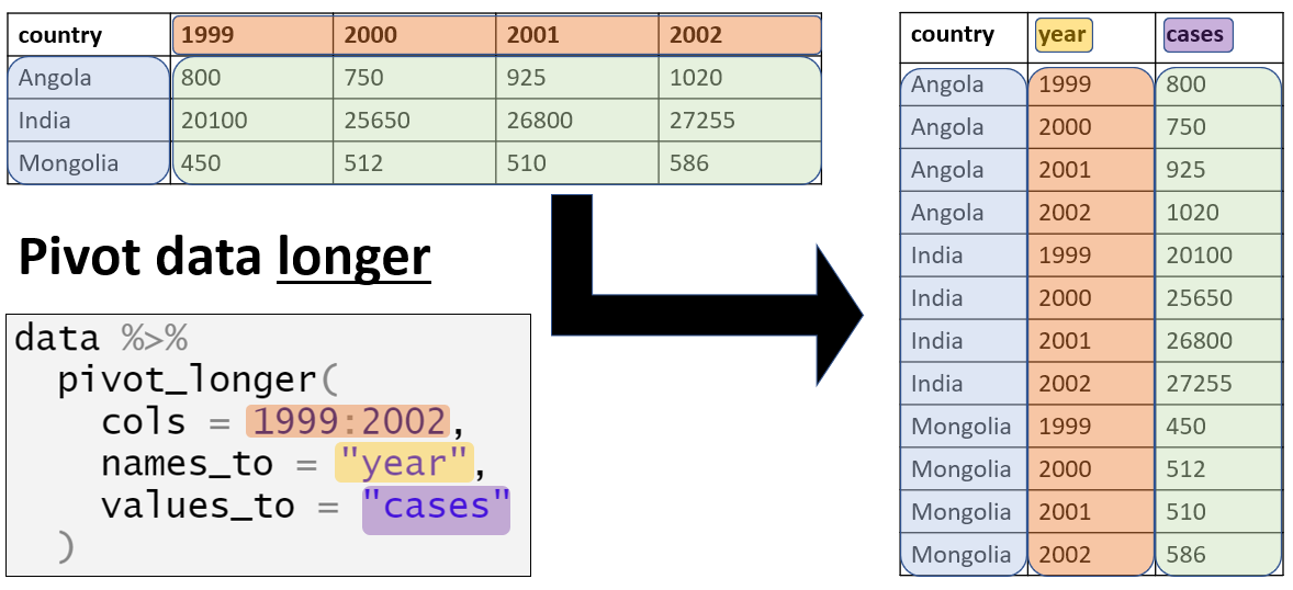
In the figure below, the data is reshaped, or made longer.

1. Notice that some columns (the first) gain repeated entries.
   
2. Also, notice that some variable names become entries in a new column.
3. Also, the old entries that are spread out in rectangular form are sent to a new column.

For more: link

Pivoting is often used to tidy data, i.e., make it look like this:

https://r4ds.hadley.nz/images/tidy-1.png

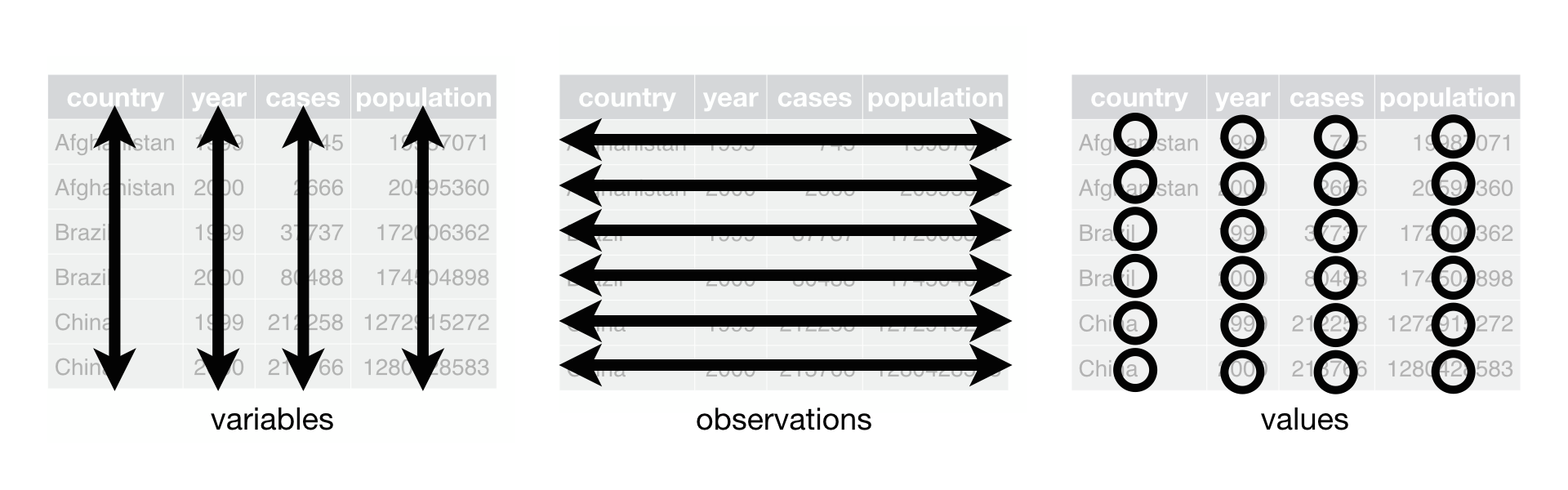
But often data is gathered in a way that is convenient for the data collector, not the data analyst.

Example

# # # # # # # # # # # # # # # # # # # # # # # # 
# 
# Assumption: df is the ATUS data after clean_names
#
# Tip: use only the data you need
d <- select(df,starts_with("act"),sex,age)

# Another tip: make a new variable that keeps track of row numbers
d <- d |> mutate(person = row_number(age))

print(d)

# A tibble: 868,270 × 6
   act_social act_sports act_work        sex        age person
        <dbl>      <dbl>    <dbl> <hvn_lbll> <hvn_lbll>  <int>
 1          0          0      910          2         30 136179
 2          0          0      910          2         30 136180
 3          0          0      910          2         30 136181
 4          0          0      910          2         30 136182
 5          0          0      910          2         30 136183
 6          0          0      910          2         30 136184
 7          0          0      910          2         30 136185
 8          0          0      910          2         30 136186
 9          0          0      910          2         30 136187
10          0          0      910          2         30 136188
# ℹ 868,260 more rows

Stack the three minute-per-activity variables into one variable of minutes and one variable of activity type.

d_pivoted <- d |> pivot_longer(
  starts_with("act_"), 
  names_to = "activity", 
  values_to = "minutes")

Group the pivoted data by sex & activity then find the total minutes on each activity for each sex

d_grouped <- group_by(d_pivoted,sex,activity) |> 
  summarize(min = sum(minutes, na.rm = TRUE))

Make a (stacked) bar chart colored by sex, whose height tracks the number of minutes

for each activity.

d_grouped |> ggplot(
  aes(x=activity, y = min, fill = haven::as_factor(sex)))  + 
  geom_bar(stat = "identity")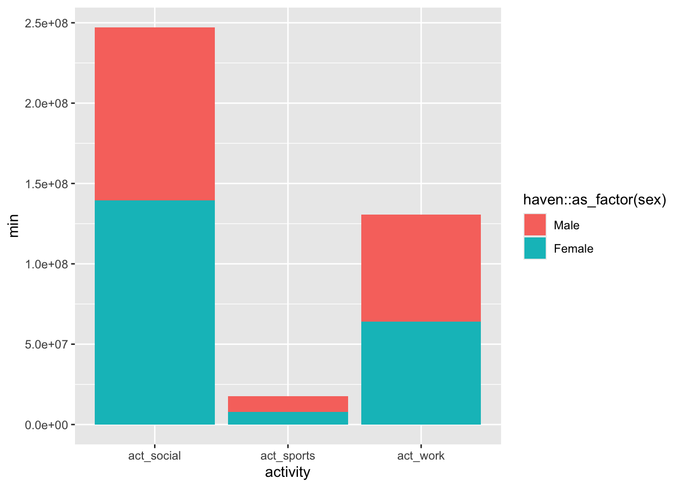

Repeat the plot above but with the bars not stacked.

d_grouped |> ggplot(aes(x=activity, y = min, fill = haven::as_factor(sex)))  + geom_bar(stat = "identity", position = "dodge")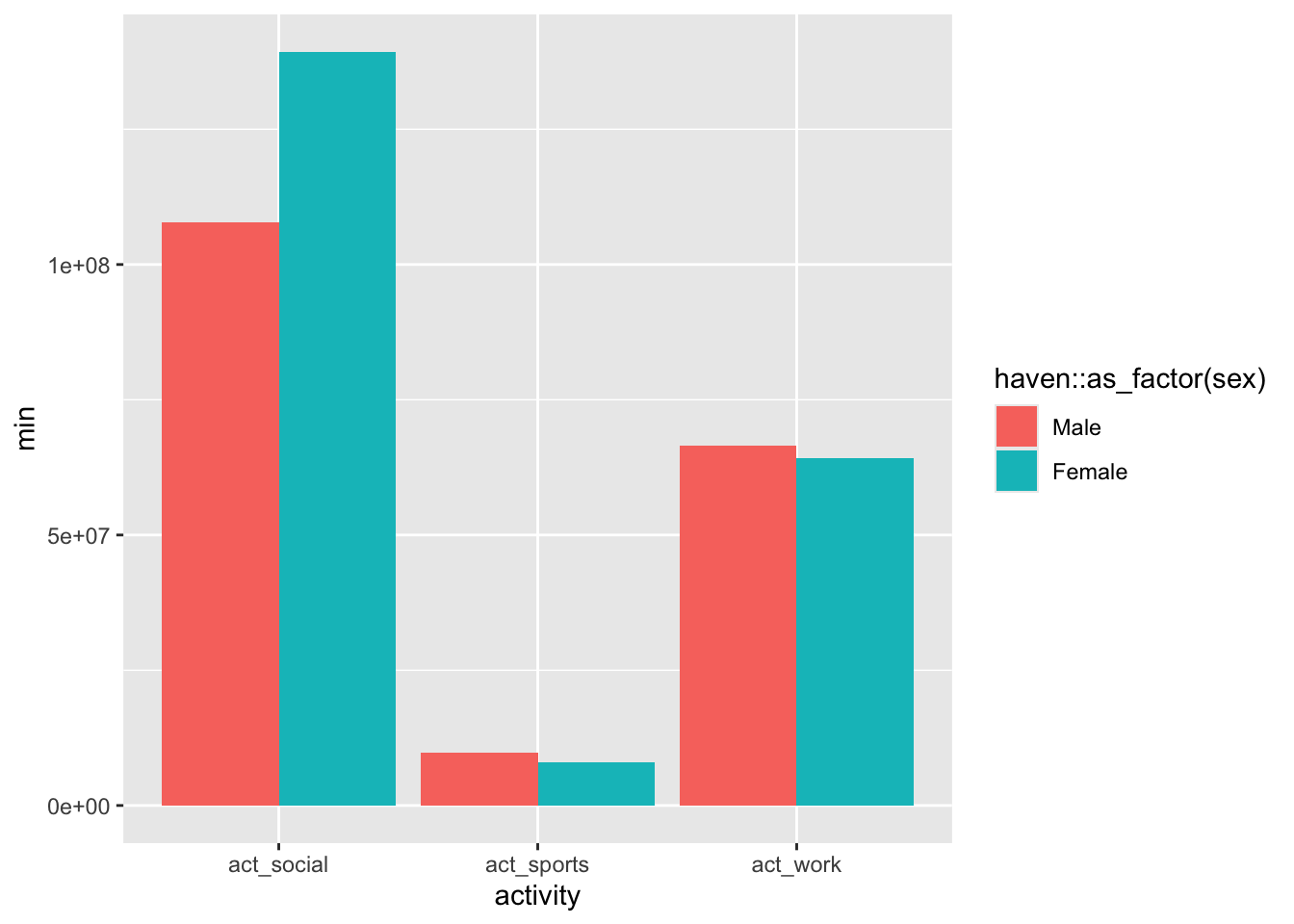

Spread a pair of columns onto a field of cells

The data in table2 is not tidy. Make it tidy with pivot_wider.

library(tidyverse)
table2

# A tibble: 12 × 4
   country      year type            count
   <chr>       <dbl> <chr>           <dbl>
 1 Afghanistan  1999 cases             745
 2 Afghanistan  1999 population   19987071
 3 Afghanistan  2000 cases            2666
 4 Afghanistan  2000 population   20595360
 5 Brazil       1999 cases           37737
 6 Brazil       1999 population  172006362
 7 Brazil       2000 cases           80488
 8 Brazil       2000 population  174504898
 9 China        1999 cases          212258
10 China        1999 population 1272915272
11 China        2000 cases          213766
12 China        2000 population 1280428583

table2 |> pivot_wider(names_from = type, values_from = count)

# A tibble: 6 × 4
  country      year  cases population
  <chr>       <dbl>  <dbl>      <dbl>
1 Afghanistan  1999    745   19987071
2 Afghanistan  2000   2666   20595360
3 Brazil       1999  37737  172006362
4 Brazil       2000  80488  174504898
5 China        1999 212258 1272915272
6 China        2000 213766 1280428583

The data in table4a is not tidy as well.

table4a |> print()

# A tibble: 3 × 3
  country     `1999` `2000`
  <chr>        <dbl>  <dbl>
1 Afghanistan    745   2666
2 Brazil       37737  80488
3 China       212258 213766

Make it tidy with pivot_longer.

By default, the new column names will be titled `name` and `value`.  The `name` variable contains the old variable names.  The `value` variable contains the old values.  Change them with:`

# Split a string into columns

Table 3 has two variables occupying a single cell.  
::: {.cell}

```{.r .cell-code}
print(table3)

# A tibble: 6 × 3
  country      year rate             
  <chr>       <dbl> <chr>            
1 Afghanistan  1999 745/19987071     
2 Afghanistan  2000 2666/20595360    
3 Brazil       1999 37737/172006362  
4 Brazil       2000 80488/174504898  
5 China        1999 212258/1272915272
6 China        2000 213766/1280428583

:::

We spread them out into two columns.

table3 |> separate_wider_delim(cols = rate,delim = "/", names = c("cases","pop"))

# A tibble: 6 × 4
  country      year cases  pop       
  <chr>       <dbl> <chr>  <chr>     
1 Afghanistan  1999 745    19987071  
2 Afghanistan  2000 2666   20595360  
3 Brazil       1999 37737  172006362 
4 Brazil       2000 80488  174504898 
5 China        1999 212258 1272915272
6 China        2000 213766 1280428583