# read_data contains read_dta
  library(haven)
  library(tidyverse)
  library(cowplot)
library(ggridges) Aesthetic & Geometric Mappings
EDA w/ Tattoo data
Tattoo Study
We use data from a study on tattoos and impulsiveness. link.
Note
There is no readme or label description for this dataset, so we’ll have to use our best guess as to what each variable means.
From the authors
Frederick (2005) developed the cognitive-reflection task (CRT), three questions designed to test subjects’ ability to overcome the intuitive but incorrect answer in order to think through the problem to arrive at the correct answer. Poor performance on the CRT has come to be interpreted as an indication of impulsiveness and predicts a wide range of behaviors, including low trust (Corgnet et al., 2016), susceptibility to the base-rate fallacy and other cognitive biases that involve a correct solution (Hoppe and Kusterer, 2011). Most relevant for our study, Frederick (2005) and Oechssler et al. (2009) both find that subjects with higher CRT scores are more likely than low-CRT subjects to choose a later, larger reward over the more immediate, smaller reward.
Because the decision to get a permanent-ink tattoo, particularly a visible tattoo, may have been made impulsively with little thought given to future employment consequences, we hypothesize that a tattoo will be associated with fewer correctly answered CRT questions.
Expoloratory Data Analysis
From Chapter 11:
Generate questions about your data.
Search for answers by visualizing, transforming, and modelling your data.
Use what you learn to refine your questions and/or generate new questions.
Load data, examine variable names & view variables that include “tat”.
# load data from Week 5 folder
tat <- read_dta("https://euclid.nmu.edu/~joshthom/teaching/dat309/week4/tattoo_dataset.dta")

# get variable names
tat_vars <- names(tat)

# select variables involving the phrase tat
tat |> select(contains("tat")) |> glimpse()
Rows: 1,104
Columns: 54
$ us_state <chr> "New York", "Missouri", "West Virginia", "Texas", "Ge…
$ tattoo <dbl+lbl> 1, 0, 0, 0, 0, 1, 0, 0, 0, 0, 0, 1, 0, 0, 0, 1, 0…
$ tat_now <dbl> 4, 0, 0, 0, 0, 1, 0, 0, 0, 0, 0, 8, 0, 0, 0, 2, 0, 0,…
$ tat_hidden <dbl> 4, 0, 0, 0, 0, 1, 0, 0, 0, 0, 0, 4, 0, 0, 0, 2, 0, 0,…
$ tat_vis <dbl> 0, 0, 0, 0, 0, 0, 0, 0, 0, 0, 0, 4, 0, 0, 0, 0, 0, 0,…
$ tat_time <dbl+lbl> 2, NA, NA, NA, NA, 3, NA, NA, NA, NA, NA, 3, N…
$ tat_last <dbl+lbl> 1, NA, NA, NA, NA, 3, NA, NA, NA, NA, NA, 4, N…
$ remove_tat <dbl> 0, NA, NA, NA, NA, 0, NA, NA, NA, NA, NA, 0, NA, NA, …
$ thinktat_n <dbl> NA, 3, 3, 3, 3, NA, 3, 3, 3, 3, 3, NA, 3, 3, 3, NA, 3…
$ temptat <dbl> 2, 3, 2, 3, 2, 2, 2, 3, NA, 2, NA, 2, 2, 2, 2, 2, 3, …
$ perc_friends_tat <dbl> 37, 19, 60, 10, 23, 69, 50, 10, 10, 25, 5, 37, 10, 22…
$ tattoo_status <dbl+lbl> 1, 0, 0, 0, 0, 1, 0, 0, 0, 0, 0, 2, 0, 0, 0, 1, 0…
$ friend_tat <dbl> 37, 19, 60, 10, 23, 69, 50, 10, 10, 25, 5, 37, 10, 22…
$ us_tat <dbl> 58, 37, 40, 15, 21, 83, 31, 18, 20, 53, 60, 19, 15, 3…
$ Gtattoo_vis <dbl> 0, 0, 0, 0, 0, 0, 0, 0, 0, 0, 0, 1, 0, 0, 0, 0, 0, 0,…
$ Gtattoo_hid <dbl> 1, 0, 0, 0, 0, 1, 0, 0, 0, 0, 0, 0, 0, 0, 0, 1, 0, 0,…
$ Gtattoo_no <dbl> 0, 1, 1, 1, 1, 0, 1, 1, 1, 1, 1, 0, 1, 1, 1, 0, 1, 1,…
$ tattoo_NHV <dbl> 1, 0, 0, 0, 0, 1, 0, 0, 0, 0, 0, 2, 0, 0, 0, 1, 0, 0,…
$ tat2_now <dbl> 16, 0, 0, 0, 0, 1, 0, 0, 0, 0, 0, 64, 0, 0, 0, 4, 0, …
$ T_likelyTat <dbl> 0, 0, 0, 0, 0, 0, 0, 0, 0, 0, 0, 0, 0, 0, 0, 0, 0, 0,…
$ T_likelynoTat <dbl> 0, 0, 0, 0, 0, 0, 0, 0, 0, 0, 0, 0, 0, 0, 0, 0, 0, 0,…
$ freq_notattoo00 <dbl> NA, NA, NA, NA, NA, NA, NA, NA, NA, NA, NA, NA, NA, N…
$ freq_notattoo01 <dbl> NA, NA, NA, NA, NA, NA, NA, NA, NA, NA, NA, NA, NA, N…
$ freq_notattoo02 <dbl> NA, NA, NA, NA, NA, NA, NA, NA, NA, NA, NA, NA, NA, N…
$ freq_notattoo03 <dbl> NA, NA, NA, NA, NA, NA, NA, NA, NA, NA, NA, NA, NA, N…
$ freq_tattoo10 <dbl> NA, NA, NA, NA, NA, NA, NA, NA, NA, NA, NA, NA, NA, N…
$ freq_tattoo11 <dbl> NA, NA, NA, NA, NA, NA, NA, NA, NA, NA, NA, NA, NA, N…
$ freq_tattoo12 <dbl> NA, NA, NA, NA, NA, NA, NA, NA, NA, NA, NA, NA, NA, N…
$ freq_tattoo13 <dbl> NA, NA, NA, NA, NA, NA, NA, NA, NA, NA, NA, NA, NA, N…
$ freq_notattoo <dbl> NA, NA, NA, NA, NA, NA, NA, NA, NA, NA, NA, NA, NA, N…
$ freq_tattoo <dbl> NA, NA, NA, NA, NA, NA, NA, NA, NA, NA, NA, NA, NA, N…
$ freq_notat <dbl> NA, NA, NA, NA, NA, NA, NA, NA, NA, NA, NA, NA, NA, N…
$ freq_notat1 <dbl> NA, NA, NA, NA, NA, NA, NA, NA, NA, NA, NA, NA, NA, N…
$ freq_notat00 <dbl> NA, NA, NA, NA, NA, NA, NA, NA, NA, NA, NA, NA, NA, N…
$ freq_tat10 <dbl> NA, NA, NA, NA, NA, NA, NA, NA, NA, NA, NA, NA, NA, N…
$ tat_3time <dbl+lbl> 1, NA, NA, NA, NA, 1, NA, NA, NA, NA, NA, 1, N…
$ tat_TimeV <dbl+lbl> NA, NA, NA, NA, NA, NA, NA, NA, NA, NA, NA, 3, N…
$ tat_TimeH <dbl+lbl> 2, NA, NA, NA, NA, 3, NA, NA, NA, NA, NA, NA, N…
$ tat_3last <dbl> 1, NA, NA, NA, NA, 2, NA, NA, NA, NA, NA, 2, NA, NA, …
$ tat_over40 <dbl> 0, 0, 0, 0, 0, 0, 0, 0, 0, 0, 0, 1, 0, 0, 0, 0, 0, 0,…
$ tat_under40 <dbl> 1, 0, 0, 0, 0, 1, 0, 0, 0, 0, 0, 0, 0, 0, 0, 1, 0, 0,…
$ tat_last20 <dbl> 0, NA, NA, NA, NA, 0, NA, NA, NA, NA, NA, 0, NA, NA, …
$ time_ustat <dbl> 638, 407, 280, 135, 126, 581, 186, 162, 40, 106, 540,…
$ timelo_ustat <dbl> 0, 0, 0, 0, 21, 0, 31, 0, 20, 53, 0, 19, 15, 0, 0, 45…
$ timehi_ustat <dbl> 58, 37, 40, 15, 0, 83, 0, 18, 0, 0, 60, 0, 0, 31, 25,…
$ ustat_over <dbl> 1, 0, 0, 0, 0, 1, 0, 0, 0, 1, 1, 0, 0, 0, 0, 1, 0, 0,…
$ us_tat2 <dbl> 3364, 1369, 1600, 225, 441, 6889, 961, 324, 400, 2809…
$ timelo_friendtat <dbl> 0, 0, 0, 0, 23, 0, 50, 0, 10, 25, 0, 37, 10, 0, 0, 50…
$ tattooed_likely <dbl> 0, 0, 0, 0, 0, 0, 0, 0, 0, 0, 0, 0, 0, 0, 0, 0, 0, 0,…
$ tat_likely <dbl> 3, 1, 1, 1, 1, 3, 1, 1, 1, 1, 1, 5, 1, 1, 1, 3, 1, 1,…
$ avg_tatlast <dbl> 0, NA, NA, NA, NA, 6, NA, NA, NA, NA, NA, 15, NA, NA,…
$ age_1tat <dbl> NA, NA, NA, NA, NA, 30, NA, NA, NA, NA, NA, NA, NA, N…
$ toss2notat <dbl> 0, 3, 3, 4, 3, 0, 3, 5, 3, 2, 3, 0, 3, 3, 3, 0, 2, 5,…
$ age40tattoo <dbl> 0, 0, 0, 0, 0, 0, 0, 0, 0, 0, 0, 1, 0, 0, 0, 0, 0, 0,…The tattoo variable indicates who has a tattoo and who does not.
# count number of people with a tatoo
tat |> group_by(tattoo) |> summarize(n = n())
# A tibble: 2 × 2
tattoo n
<dbl+lbl> <int>
1 0 [No Tattoo] 781
2 1 [Tattoo] 323The occu contains occupations, and Teacher is different from `teacher. So we fix this. How are tattoos distributed among occupations?
Notice the fct_reorder reorders the x-axis for better readability.
tat <- mutate(tat, occu = factor(tolower(occu)))

tat_occu <- tat |> group_by(tattoo,occu) |> summarize(n = n()) |> arrange(-n)

tat_occu |> filter(n > 5) |>
  ggplot(aes(
    x=fct_reorder(occu,-n),
    y = n,
    fill = as.factor(tattoo))) +
  geom_col(position = "dodge") +
  coord_flip()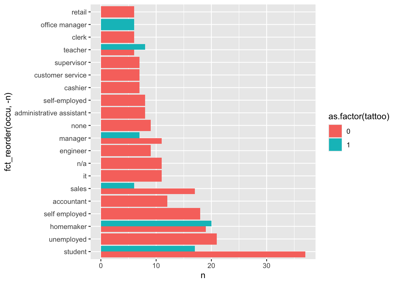
Replacing the barplot with lollipop chart
# attempt 1
tat_occu |> filter(n > 5, tattoo == 1) |>
  ggplot(aes(
    y=occu,
    x = n,
    fill = as.factor(tattoo))) +
  # this creates the stick
  geom_segment(aes(
    y = occu,
    yend = occu,
    x = 0,
    xend = n)) +
  # makes the circle
  geom_point(aes(
    fill = as.factor(tattoo)),
    shape = 21, size = 5,
    stroke = 1, color = "black", alpha = .7,
    show.legend = FALSE) +
  labs(x = "Number of People", y = "Occupation", title = "Occupations & Tattoos") +
    theme(plot.title = element_text(size = 20, colour = "#668cff"),
        axis.title.x = element_text(size = 10, colour = "#6699ff"),
        axis.title.y = element_text(size = 10, colour = "#ff8080")) +
  # add vertical grid to plot
  # play around with where this is within the plotting function
theme_minimal_vgrid() 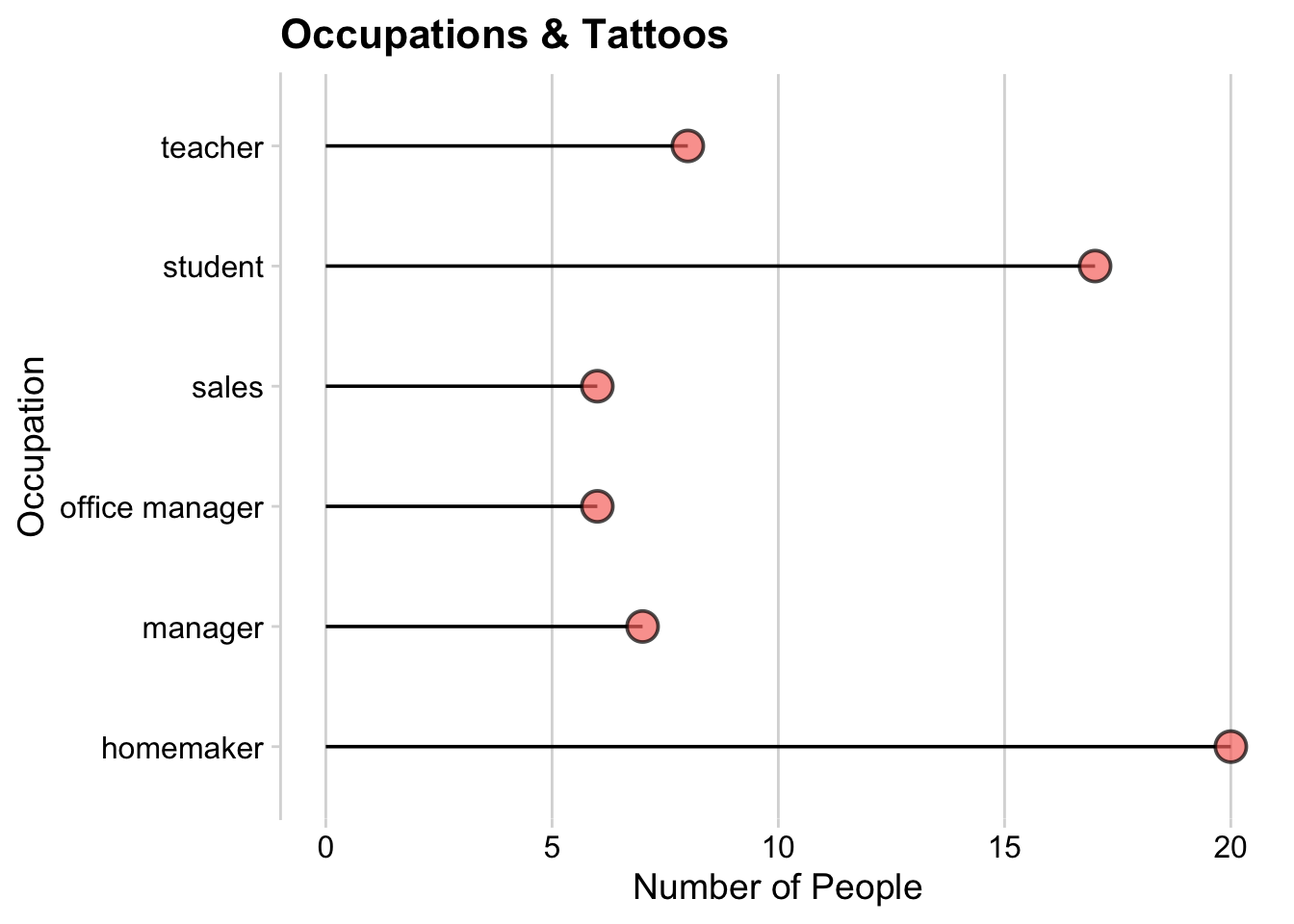
Improve the plot by:
# attempt 2
tat_occu |> filter(n > 5, tattoo == 1) |>
  ggplot(aes(
    y=fct_reorder(occu,-n),
    x = n,
    fill = as.factor(tattoo))) +
  geom_segment(aes(y = fct_reorder(occu,-n),
    yend = fct_reorder(occu,-n),
    x = 0,
    xend = n)) +
  geom_point(aes(
    fill = as.factor(tattoo)),
    shape = 21, size = 5, stroke = 1, color = "black", alpha = .7,
    show.legend = FALSE) +
  labs(x = "Number of People", y = "Occupation", title = "Occupations & Tattoos") +
    theme(plot.title = element_text(size = 20, colour = "#668cff"),
        axis.title.x = element_text(size = 10, colour = "#6699ff"),
        axis.title.y = element_text(size = 10, colour = "#ff8080")) +
  # add vertical grid to plot
theme_minimal_vgrid() 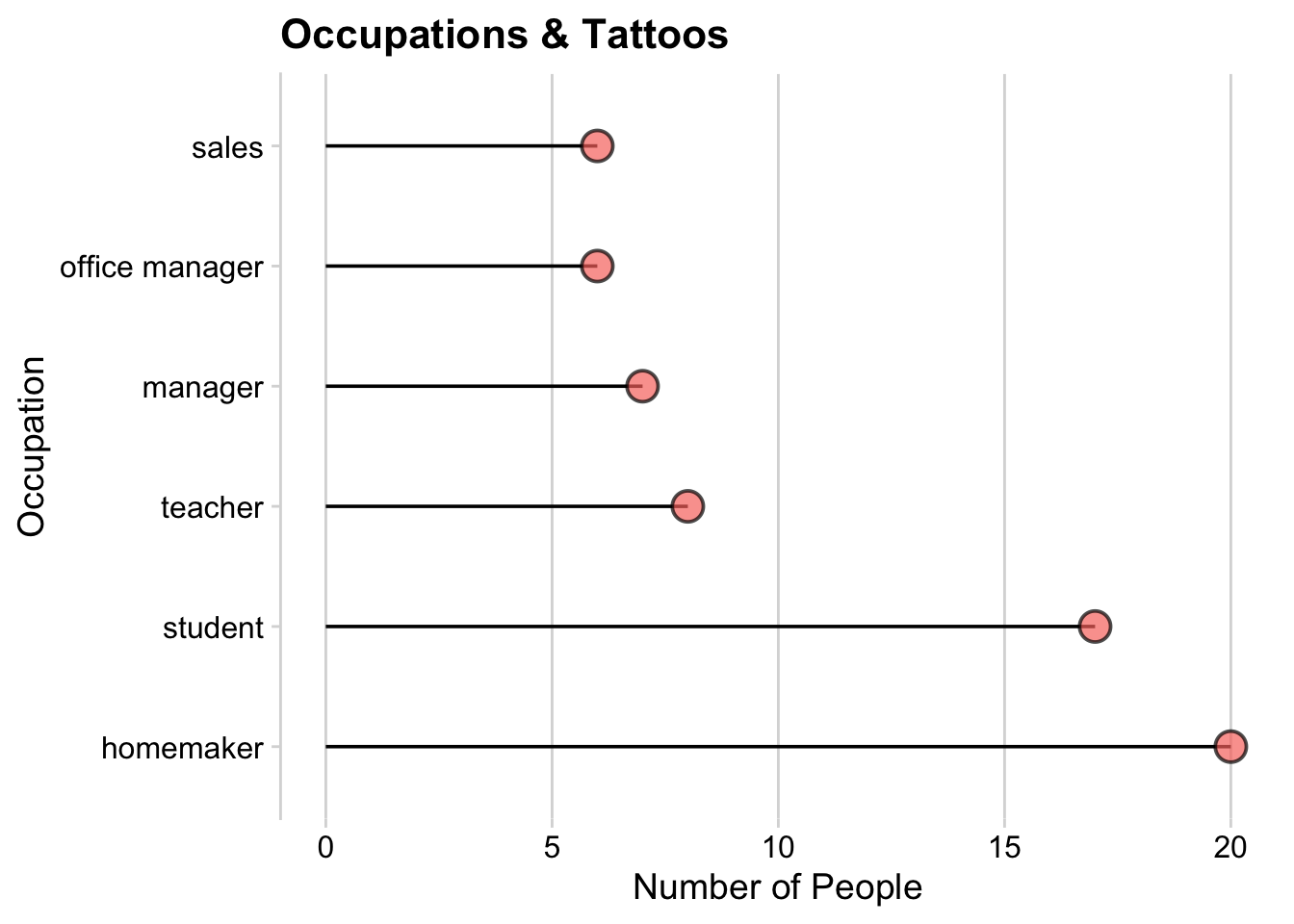
But maybe this was too many times to use fct_reorder …
# Improve the code above using
# mutate to make the occu variable an factor ordered by frequency
tat_occu <- tat_occu |> mutate(occu = fct_reorder(occu,-n))
Search for variables of a particular type.
  # find other categorical variables
  tat |> select(!where(is.numeric))
# A tibble: 1,104 × 28
v1 v8 v9 q158 gender_text marital_text ethnicity_text country
<chr> <chr> <chr> <chr> <chr> <chr> <chr> <chr>
1 R_6sclDq7G… 10/0… 10/0… A3OG… "" "" "" usa
2 R_1mVND2VH… 10/0… 10/0… A1FY… "" "" "" United…
3 R_uexTUNVZ… 9/30… 9/30… AYPR… "" "" "" USA
4 R_dgoT4Y9L… 10/0… 10/0… AX31… "" "" "" USA
5 R_2sT6OIAh… 9/29… 9/29… A35L… "" "" "" US
6 R_71lyMZ2L… 10/0… 10/0… A2FB… "" "" "" US
7 R_3iX1YeLe… 10/1… 10/1… A1A3… "" "" "" USA
8 R_2saNqCpw… 10/1… 10/1… A1CH… "" "" "" usa
9 R_2uTDN5Qg… 08/0… 08/0… A26U… "" "" "" usa
10 R_0GSMEgqi… 9/30… 9/30… A132… "" "" "" india
# ℹ 1,094 more rows
# ℹ 20 more variables: us_state <chr>, occu <fct>, mthr_occu <chr>,
# fthr_occu <chr>, crt_4_1_text <chr>, rel_raised_text <chr>,
# rel_curren_text <chr>, denom_text <chr>, notes <chr>, onum_y <chr>,
# whyhide_other_text <chr>, whyvisibl_other_text <chr>,
# drawback_y_7_text <chr>, procon_y_14_text <chr>, procon2_y_14_text <chr>,
# consid_n_12_text <chr>, procon_n_14_text <chr>, startdatetime <date>, … tat |> ggplot(aes(x=alcohol, y = smoke, color = as.factor(tattoo))) + geom_point(position = "jitter")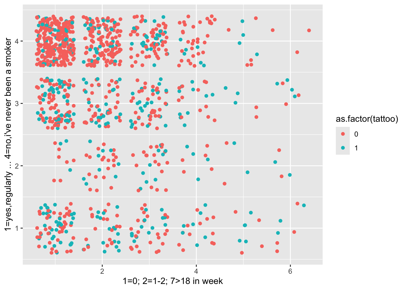
tat |> group_by(tattoo, smoke) |> summarize(m = mean(alcohol)) |>
ggplot(aes(x=smoke,y=m,group = tattoo,fill = as_factor(tattoo))) + geom_col(position = "dodge") 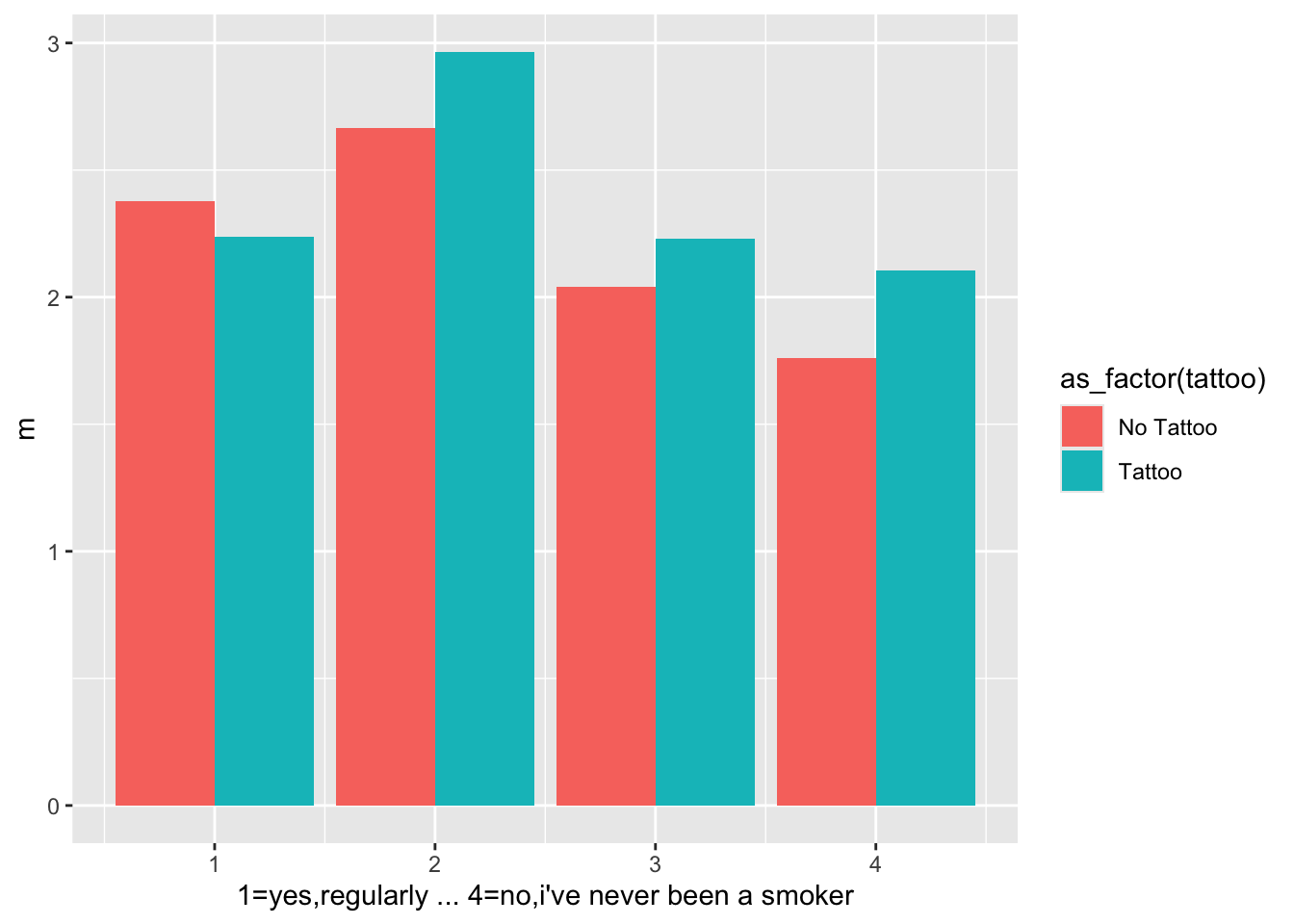
  # notice the negative sign
  p <- tat |> ggplot(aes(x=alcohol, y = smoke, color = as.factor(tattoo))) + geom_smooth()

# what happens when you remove this
suppressWarnings(print(p))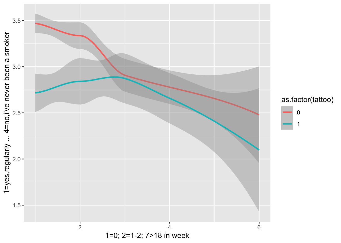
tat |> ggplot(aes(x=smoke, y = ave_health, color = as.factor(tattoo))) + geom_smooth()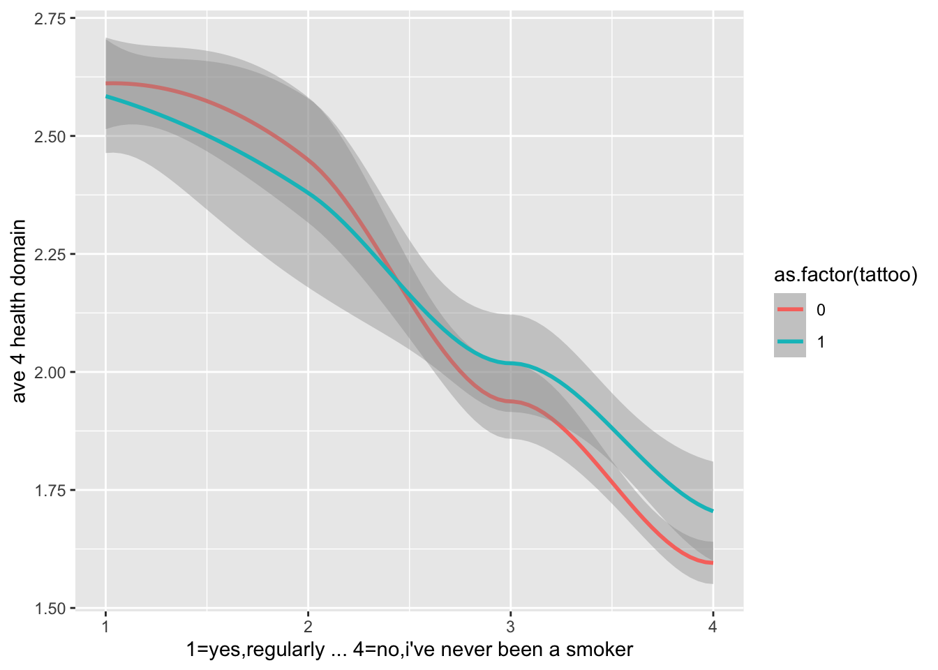
tat |> ggplot(aes(x=alcohol, y = ave_health, color = as.factor(tattoo))) + geom_smooth()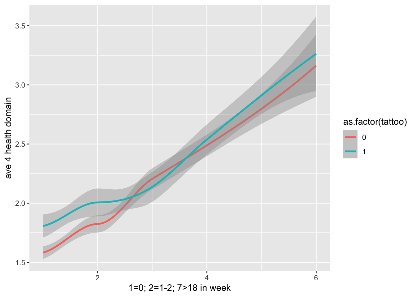
tat |> ggplot(aes(x = factor(tattoo), fill = factor(CRT2_correct))) + geom_bar()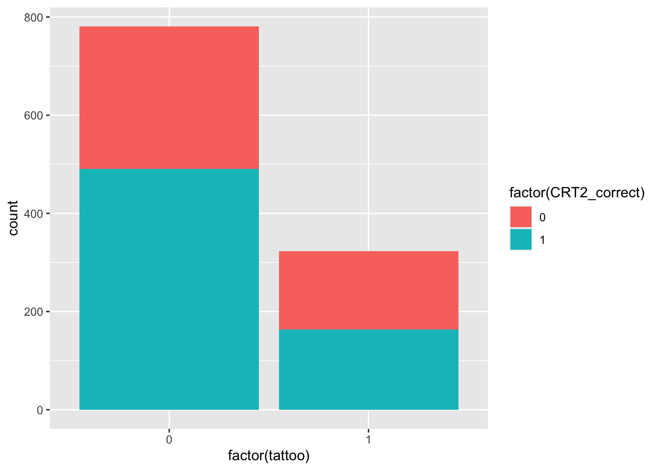
   tat |> ggplot(aes(
     x = factor(cut(tat_vis,breaks = c(-1,0,1,50))),
     fill = factor(CRT2_correct))) +
     geom_bar(position = "fill") +
     scale_x_discrete(
       name = "Number of Tattoos",
       labels = c("0","1","Multiple"))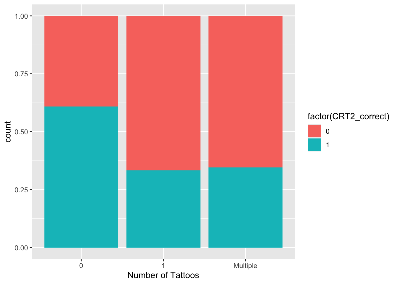
  # tattoos vs. alcohol
  tat |> ggplot(aes(y = factor(tattoo), x = alcohol)) + geom_density_ridges()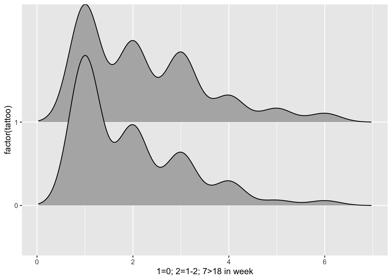
Tattoos & Crowd-funding
This study seems interesting but their data is only available upon request. It might be good for a subsequent project.