library(tidyverse)
library(tidyquant) # contains coord_x_datetime for dates as coordinates
library(scales)Load & Wrangle Zillow Data
Intro loops & functions
Library load
This data, from Zillow, comes to us in two files; one associated with yts (zillow home value index) and one with nrin (total monthly payment). We well join the datasets together so that each house is an observation and nrin and yts are variables.
0. load data
# Years to Save: A measure of the number of years it would take the median household to save for a 20% down payment on a home, assuming they are able to save 10% of their income into a simple savings account accruing no interest. This is equivalent to the number of years it would take the median household to save for a 10% down payment, assuming a 5% savings rate.
yts <- read_csv("https://euclid.nmu.edu/~joshthom/teaching/dat309/week8/Metro_years_to_save_downpayment_0.20_uc_sfrcondo_tier_0.33_0.67_sm_sa_month.csv") |> janitor::clean_names()

# New Renter Income Needed: An estimate of the household income required to spend less than 30% of monthly income to newly lease the typical rental.
nrin <- read_csv("https://euclid.nmu.edu/~joshthom/teaching/dat309/week8/Metro_new_renter_income_needed_uc_sfrcondomfr_sm_sa_month.csv") |> janitor::clean_names()

print(yts, n = 5)
# A tibble: 390 × 169
region_id size_rank region_name region_type state_name x2012_01_31 x2012_02_29
<dbl> <dbl> <chr> <chr> <chr> <dbl> <dbl>
1 102001 0 United Sta… country <NA> 6.30 6.28
2 394913 1 New York, … msa NY 11.4 11.4
3 753899 2 Los Angele… msa CA 13.0 12.9
4 394463 3 Chicago, IL msa IL 5.83 5.78
5 394514 4 Dallas, TX msa TX 4.99 4.99
# ℹ 385 more rows
# ℹ 162 more variables: x2012_03_31 <dbl>, x2012_04_30 <dbl>,
# x2012_05_31 <dbl>, x2012_06_30 <dbl>, x2012_07_31 <dbl>, x2012_08_31 <dbl>,
# x2012_09_30 <dbl>, x2012_10_31 <dbl>, x2012_11_30 <dbl>, x2012_12_31 <dbl>,
# x2013_01_31 <dbl>, x2013_02_28 <dbl>, x2013_03_31 <dbl>, x2013_04_30 <dbl>,
# x2013_05_31 <dbl>, x2013_06_30 <dbl>, x2013_07_31 <dbl>, x2013_08_31 <dbl>,
# x2013_09_30 <dbl>, x2013_10_31 <dbl>, x2013_11_30 <dbl>, …print(nrin, n = 5) # A tibble: 390 × 133
region_id size_rank region_name region_type state_name x2015_01_31 x2015_02_28
<dbl> <dbl> <chr> <chr> <chr> <dbl> <dbl>
1 102001 0 United Sta… country <NA> 48274. 48494.
2 394913 1 New York, … msa NY 96056. 96695.
3 753899 2 Los Angele… msa CA 72210. 72589.
4 394463 3 Chicago, IL msa IL 56512. 56572.
5 394514 4 Dallas, TX msa TX 43984. 44136.
# ℹ 385 more rows
# ℹ 126 more variables: x2015_03_31 <dbl>, x2015_04_30 <dbl>,
# x2015_05_31 <dbl>, x2015_06_30 <dbl>, x2015_07_31 <dbl>, x2015_08_31 <dbl>,
# x2015_09_30 <dbl>, x2015_10_31 <dbl>, x2015_11_30 <dbl>, x2015_12_31 <dbl>,
# x2016_01_31 <dbl>, x2016_02_29 <dbl>, x2016_03_31 <dbl>, x2016_04_30 <dbl>,
# x2016_05_31 <dbl>, x2016_06_30 <dbl>, x2016_07_31 <dbl>, x2016_08_31 <dbl>,
# x2016_09_30 <dbl>, x2016_10_31 <dbl>, x2016_11_30 <dbl>, …1. rename x’s with yts and nrin, respectively
First, we rename variables to make it easier to interpret the nrin & yts price variables. We have rename_with use the str_replace function to perform a renaming of many variables at once.
- The
~syntax makesstr_replaceinto a function whose argument. - The data is sent to the
.spot.
- Thy syntax is str_replace(data, thing_to_replace, new_string)
yts <- yts |> rename_with(~str_replace(.,"x","yts_"))
nrin <- nrin |> rename_with(~str_replace(.,"x","nrin_"))
2. use names() and head() to note the 1st 10 variables
nrin |> names() |> head(n=10) [1] "region_id" "size_rank" "region_name" "region_type"
[5] "state_name" "nrin_2015_01_31" "nrin_2015_02_28" "nrin_2015_03_31"
[9] "nrin_2015_04_30" "nrin_2015_05_31"yts |> names() |> head()[1] "region_id" "size_rank" "region_name" "region_type"
[5] "state_name" "yts_2012_01_31"3. Joining 101:
There are several ways of joining two data sets together, some are illustrated below.

join two data sets with full_join
Joining two data frames using “left_join” or “right_join” requires a variable common to both data frames and keeps data. We use full_join to bring in new (non-redundant) variables.
Learn more about joining here.
nrin_yts <- full_join(yts,nrin)5. pivot to get plotable data
#
# ytsing price & nrining price are variables
zillow <- pivot_longer(nrin_yts,
                      cols = starts_with("yts"),
                      names_to = "yts_date",
                      values_to = "years_to_save") |> # before buying an avg house
  pivot_longer(
    cols = starts_with("nrin"),
    names_to = "nrin_date",
    values_to = "income_needed") # to rent @ < 30%

zillow <- zillow |>
  mutate(
    nrin_date = as_datetime(str_remove(nrin_date,"nrin_")),
    yts_date = as_datetime(str_remove(yts_date,"yts_"))
    ) |>
  relocate(nrin_date,.before=1) |>
  drop_na()
7. filter to get some reasonable sized data
# parameter "name" : vector of strings of state names: c("CO","MI")
# parameter "number" : the number of regions to pull from each states
get_states <- function(name, number){

  # empty dataset
  d <- {}
  for (i in 1:length(name)){
    # print the name of the state for sanity
    print(name[i])

    # get all data for the given name
    my_states <- filter(zillow, state_name %in% name[i])

    # grab a few region_names from each state
    some_names <- distinct(my_states,region_name) |>
      slice_sample(n = number)

    some_regions <- filter(my_states,
                           region_name %in% pull(some_names))
    # could also do some_names[[1]] to extract the vector from the tibble

    d <- bind_rows(d,some_regions)
  }
  return(d)
}

zil_sub <- get_states(c("NC","MI","NY","WA", "WY"),3)
[1] "NC"
[1] "MI"
[1] "NY"
[1] "WA"
[1] "WY"8. plot years to save before buyint average home for each region
p <- ggplot(zil_sub, aes(x = yts_date, y = years_to_save,
                         group = region_name,
                         color = region_name)) + geom_line()

print(p)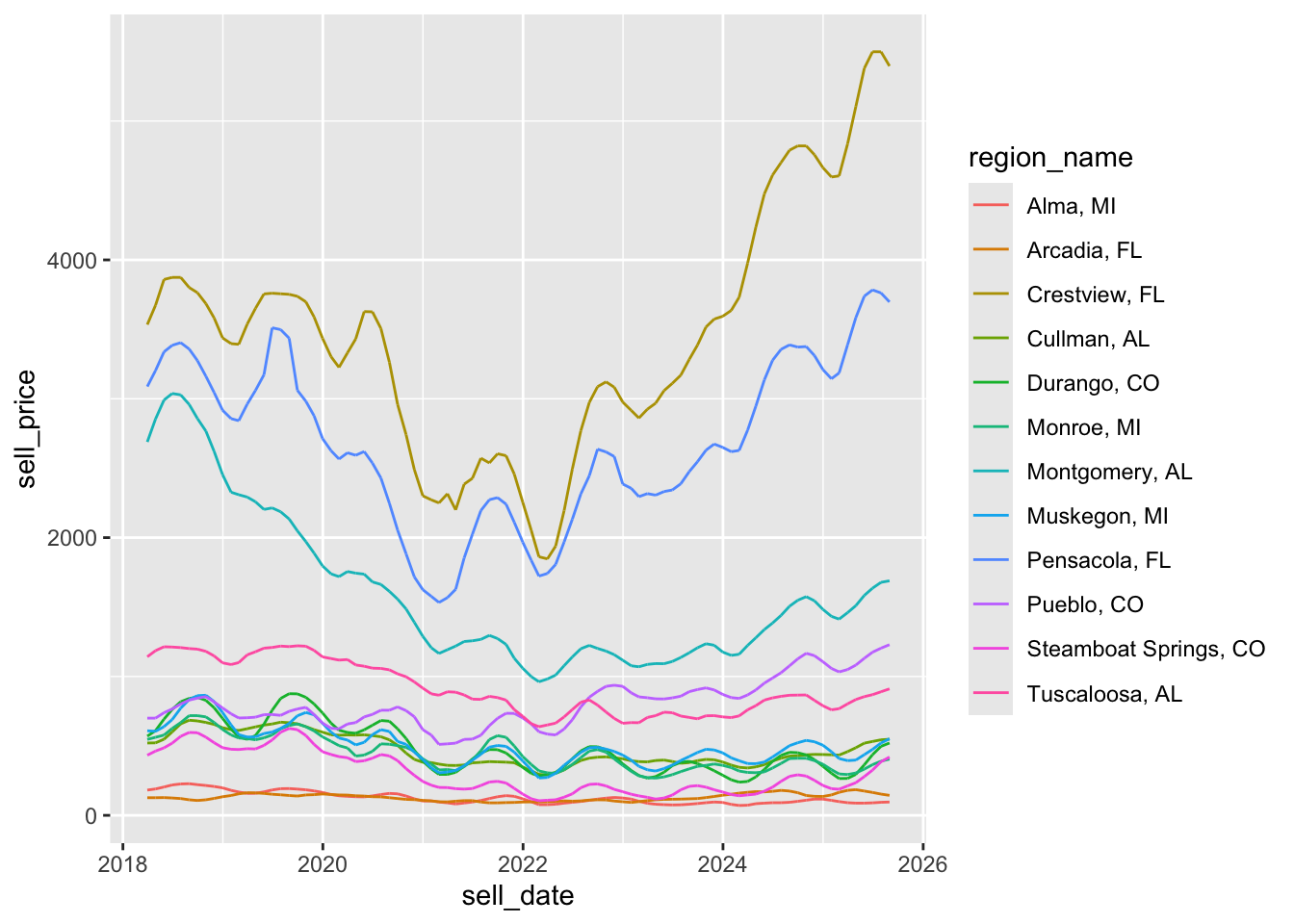
9. Plot income needed so that an average rental costs less than 30% of your income for each region
# option 1: plot alongside the yts plot
q <- ggplot(zil_sub, aes(x = nrin_date, y = income_needed,
                         group = region_name,
                         color = region_name)) + geom_line()

print(q)
Note that the as_date() or as_datetime() functions can be used to cast strings into variables of type date or dttm
str <- "2019-01-01 00:14:15"
as_datetime(str)
[1] "2019-01-01 00:14:15 UTC"This works a bit ebetter:
p <- ggplot(zil_sub, aes(x = nrin_date, y = income_needed,
                         group = region_name,
                         color = region_name,
                         linetype = state_name)) +
      geom_line()
This is even better:
# zoom to the interesting region
p + scale_x_date(date_breaks = "2 years")
#p + coord_x_datetime(xlim = c("2018-01-01", "2023-12-31")) # even better still
p + scale_x_date(date_breaks = "1 year", date_labels= "%Y")
Zoom in on post 2018. Here we use coord_x_date to showcase how to zoom without losing data. (The coord_ functions allow for zooming without removing data that might be used to compute a statistic)
p + scale_x_date(
  date_breaks = "1 year",
  date_labels= "%Y") +
  theme(axis.text.x = element_text(size = 5)) +
  coord_x_date(xlim = c("2018-01-01","2024-01-01"))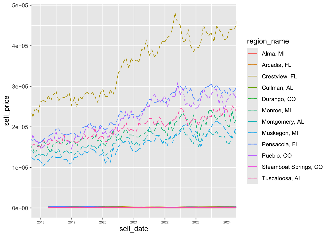
Get better formatting on the y-axis
p + scale_x_date(
      date_breaks = "1 year",
      date_labels= "%Y") +
    theme(axis.text.x = element_text(size = 5)) +
    labs(x = "Year", y = "Income Needed to Buy Average Home") +
    scale_y_continuous(label = label_dollar(prefix = "$"))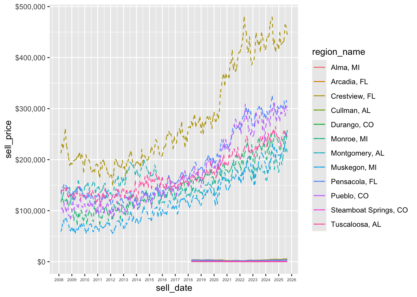
10. zoom to the interesting region
p + scale_x_date(
      date_breaks = "1 year",
      date_labels= "%Y",
      limits =
      c(as_date("2018-01-01"), as_date("2023-12-31")))  +
    theme(axis.text.x = element_text(size = 5)) +
    scale_y_continuous(label = label_dollar(prefix = "$")) +
    labs(title = "Income Needed",
    subtitle = "To Lease an Average Rental")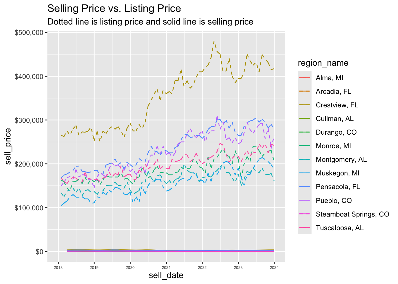
Save data for future work
This saves the variable zil_sub to the filename indicated below. Load it back up in R with load("zillow-data.Rdata").
write_rds(zil_sub, file = "~/t/dat309/week7/zillow-data.Rdata")