Zillow Map

Coloring Counties with Data

Load Zillow Data

On the Zillow Data page, one can download ZHVI data for each county in the US. Data for 2025 was saved in the week9 folder. Import below:

library(tidyverse)
# load housing data for each county
zil <- read_csv("https://euclid.nmu.edu/~joshthom/teaching/dat309/week9/County_zhvi_uc_sfrcondo_tier_0.33_0.67_sm_sa_month_2025.csv")

# clean names
zil <- janitor::clean_names(zil)

Next we use the pivoting script created previously to tidy the data

Pivot the data

# one could use rowwise(), c_across(), etc but this is nicer
# 
# edit the path below to your copy of the script
source('~/t/dat309/week8/load_clean_zillow.R')

[1] "dataset yts loaded"

[1] "dataset nrin loaded"

[1] "dataset nra loaded"

# this creates a variable named value
zil_pivot <- clean_it(zil, 'value')

zil_pivot |> head()

# A tibble: 6 × 11
  region_id size_rank region_name        region_type state_name state metro     
      <dbl>     <dbl> <chr>              <chr>       <chr>      <chr> <chr>     
1      3101         0 Los Angeles County county      CA         CA    Los Angel…
2      3101         0 Los Angeles County county      CA         CA    Los Angel…
3      3101         0 Los Angeles County county      CA         CA    Los Angel…
4      3101         0 Los Angeles County county      CA         CA    Los Angel…
5      3101         0 Los Angeles County county      CA         CA    Los Angel…
6      3101         0 Los Angeles County county      CA         CA    Los Angel…
# ℹ 4 more variables: state_code_fips <chr>, municipal_code_fips <chr>,
#   date <date>, value <dbl>

Create a county fips code

The plot_usmap() function requires the fips code for plotting. The alternative is to use lat/lon pairs together with geom_polygon().

The zillow data comes with a state fips code and a municipal fips code we glue together to define a county fips code.

# still need to make a county fips code
zil_pivot <- mutate(
  zil_pivot,
  fips = as.character(
    paste0(
      state_code_fips, 
      municipal_code_fips)
  )) |> relocate(fips)

Join Zillow data with Fips data

The us_map() function creates a variable called geom used to plot a polygon representing each county.

Join the geometry data with the zillow data using the fips code.

library(usmap)
county_map_data = us_map(regions = 'counties')
cd <- inner_join(zil_pivot, county_map_data)

Find the mean home value for each county.

# summary
zil_p <- cd |> 
    group_by(region_name, state_name, fips, geom) |> 
    summarize(mean = mean(value, na.rm=TRUE)) |>
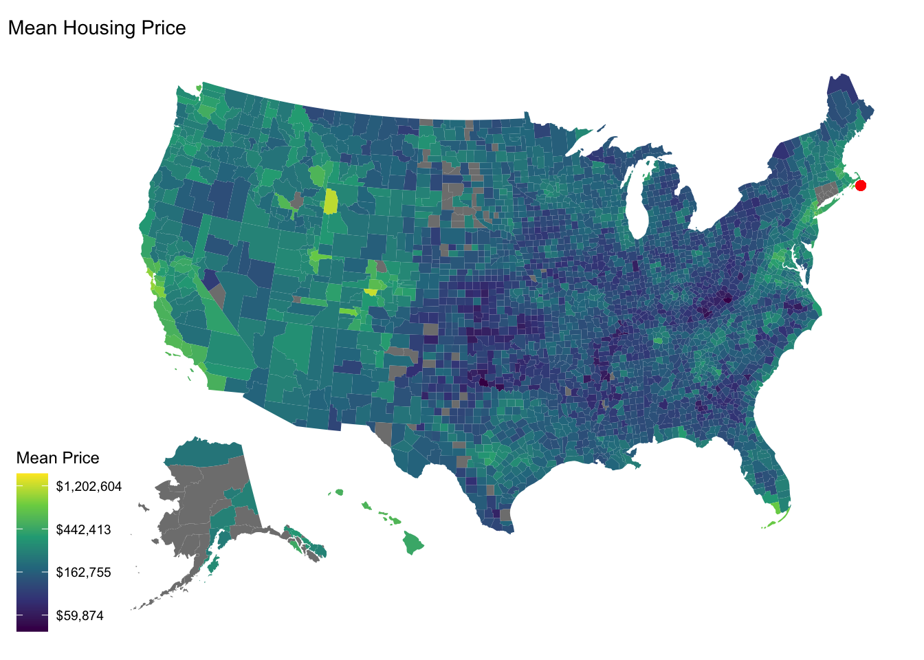
    arrange(-mean)

Map

library(scales) # for the label_dollar below

# grab lat/lon coord of center of the counties
g <- sf::st_centroid(zil_p$geom)

plot_usmap(
  data = zil_p, # the joined data
  regions = "counties", 
  values = "mean", # using the mean variable for fill color
  color = "grey90", linewidth = 0.0005) + # make the boundaries small
  labs(title = "Mean Housing Price") + 
  # trans = 'log' plots the colors on a log scale 
  # (good for large scale diffs)
  scale_fill_viridis_c(trans = "log",labels = label_dollar()) +
  # since the values = "mean" is really fill = "mean"
  labs(fill = "Mean Price") +
  # plot a red dot near the most expensive county
  geom_sf(data = filter(zil_p, mean == max(mean)),
    aes(geometry = g[1]), # plot the first centroid
    regions = 'counties',
    color = 'red', size = 2)