Siefert Van Kampen Theorem & The Classification of Surfaces
The Fundamental Group of the Klein Bottle
To compute \(\pi_1(K)\), we view the Klein bottle as a quotient of a square \(I^2\) with edges identified according to the word \(abab^{-1}\).
1. The Decomposition
Similar to the torus, we decompose \(K\) into two open sets \(U\) and \(V\):
- \(U\): The interior of the square (an open disk). \(U\) is contractible.
- \(\pi_1(U) \cong \{1\}\)
- \(V\): The 1-skeleton (the edges \(a\) and \(b\)) plus a neighborhood. \(V\) deformation retracts onto \(S^1 \vee S^1\).
- \(\pi_1(V) \cong\langle a, b\mid \emptyset\rangle\)
- \(U \cap V\): An open strip that deformation retracts onto a circle \(\gamma\).
- \(\pi_1(U \cap V) \cong \mathbb{Z}\)
2. The Amalgamated Free Product
We apply the Seifert-van Kampen Theorem:
\[\pi_1(K) \cong \pi_1(U) *_{\pi_1(U \cap V)} \pi_1(V)\]
- Map \(i_*: \pi_1(U \cap V) \to \pi_1(U)\): As \(U\) is contractible, \(i_*(\gamma) = 1\).
- Map \(j_*: \pi_1(U \cap V) \to \pi_1(V)\): Following the boundary of the square for the Klein bottle, the path is \(a\) followed by \(b\), then \(a\) again, then \(b^{-1}\).
- \(j_*(\gamma) = abab^{-1}\)
3. Calculation
The presentation for the amalgamated free product is:
\[ \pi_1(K) \cong \langle a, b\mid 1 = abab^{-1} \rangle \]
Unlike the torus, where the relation \(aba^{-1}b^{-1} = 1\) leads to an abelian group (\(\mathbb{Z}^2\)), the Klein bottle’s relation is: \[aba = b\] This group is non-abelian. It can be viewed as a semi-direct product \(\mathbb{Z} \rtimes \mathbb{Z}\), reflecting the twist in the surface’s topology.
The Real Projective Line (\(\mathbb{RP}^1\)): Topology Notes
Standard calculus treats \(+\infty\) and \(-\infty\) as distinct “directions.” In topology, \(\mathbb{RP}^1\) is the result of taking the standard real number line \(\mathbb{R}\) and “pinching” both ends together at a single point called the Point at Infinity (\(\infty\)).
- Result: \(\mathbb{RP}^1\) is topologically equivalent (homeomorphic) to a Circle (\(S^1\)).
- Key Concept: In projective space, there is only one infinity.
Geometric Construction: The Space of Lines
The most robust way to define \(\mathbb{RP}^1\) is as the set of all lines through the origin in \(\mathbb{R}^2\).
- Every line in the 2D plane passing through \((0,0)\) represents exactly one point in \(\mathbb{RP}^1\).
- The Slope Mapping: * A line with slope \(m\) corresponds to the real number \(m \in \mathbb{R}\).
- The vertical line (where slope is “undefined”) corresponds to the point \(\infty\).
- \(\mathbb{RP}^1 = \mathbb{R} \cup \{\infty\}\)
Homogeneous Coordinates
To avoid the “undefined” problem of dividing by zero, we use Homogeneous Coordinates \([x : y]\).
- A point is defined as a ratio rather than a single value.
- \([x : y]\) is the same point as \([\lambda x : \lambda y]\) for any \(\lambda \neq 0\).
- Mapping to the Real Line: * If \(y \neq 0\), the point is \([x/y : 1]\), corresponding to the standard coordinate \(x/y\).
- If \(y = 0\), the point is \([1 : 0]\), which is the formal definition of the Point at Infinity.
Visualizing the Horizon
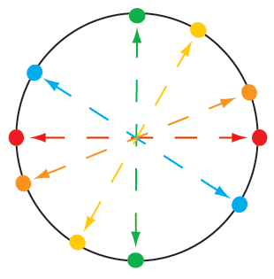
Imagine standing at the origin of a 2D plane. * Every direction you can point your finger is a “point” in the projective line. * Note that pointing “North” and “South” identifies the same line, so they represent the same point in \(\mathbb{RP}^1\). * This “identification” of opposite directions is why the projective line is a “closed” loop.
Projective Plane \(\mathbb{RP}^2\): Fundamental Group Calculation
One definition of the projective plane is the space of lines through the origin in \(\mathbb{R}^3\). Another is the quotient of the sphere \(S^2\) by the antipodal map. A third is a disk with antipodal points on the boundary identified.
In general, to define projective spaces, we take \(\mathbb{R}^{n+1} \setminus \{0\}\) and quotient by the equivalence relation \(x \sim \lambda x\) for \(\lambda \in \mathbb{R}^*\). The resulting space is \(\mathbb{RP}^n\).
The projective plane \(\mathbb{RP}^2\) can be represented as a disk with antipodal points on the boundary identified. We can decompose it into:
- \(U\): The interior of the disk (contractible).
- \(\pi_1(U) \cong \{1\}\)
- \(V\): A neighborhood of the boundary circle, which deformation retracts onto \(S^1\).
- \(\pi_1(V) \cong \mathbb{Z}\)
- \(U \cap V\): An annulus that deformation retracts onto \(S^1\).
- \(\pi_1(U \cap V) \cong \mathbb{Z}\)
Applying Seifert-van Kampen: \[\pi_1(\mathbb{RP}^2) \cong \pi_1(U) *_{\pi_1(U \cap V)} \pi_1(V)\]
- Map \(i_*: \pi_1(U \cap V) \to \pi_1(U)\): Since \(U\) is contractible, \(i_*(\gamma) = 1\).
- Map \(j_*: \pi_1(U \cap V) \to \pi_1(V)\): The loop \(\gamma\) corresponds to going around the boundary circle, which is comprised of two generators of \(\pi_1(V) \simeq \mathbb{Z}\).
- \(j_{*}(\gamma) = 2\alpha\) (where \(\alpha\) is the generator of \(\pi_1(V)\))
Thus, the presentation for \(\pi_1(\mathbb{RP}^2)\) is: \[\pi_1(\mathbb{RP}^2) \cong \langle \alpha\mid 2\alpha = 0 \rangle \cong \mathbb{Z}/2\mathbb{Z}\]
Chart of some fundamental groups of surfaces
| Surface | Symbol | Fundamental Group (\(\pi_1\)) | Euler Characteristic (\(\chi\)) |
|---|---|---|---|
| Sphere | \(S^2\) | \(0\) (Trivial) | \(2\) |
| Torus | \(T^2\) | \(\mathbb{Z} \times \mathbb{Z}\) | \(0\) |
| Genus 2 Surface | \(\Sigma_2\) | \(\langle a_1, b_1, a_2, b_2\mid [a_1, b_1][a_2, b_2] = 1 \rangle\) | \(-2\) |
| Real Projective Plane | \(\mathbb{RP}^2\) | \(\mathbb{Z}_2\) | \(1\) |
| Klein Bottle | \(K\) | \(\langle a, b\mid abab^{-1} = 1 \rangle\) | \(0\) |
Building New Surfaces From Old Ones - Connected Sums
The process of creating new surfaces by “gluing” together existing ones is called the connected sum. The connected sum of two surfaces \(M\) and \(N\), denoted \(M \# N\), is formed by removing a disk from each surface and then identifying the resulting boundary circles.
Because we are removing disks (which are contractible), the fundamental group of the connected sum can be computed using Seifert-van Kampen as the free product of the fundamental groups of the original surfaces: \[\pi_1(M \# N) \cong \pi_1(M) * \pi_1(N)\] The idea is that the “hole” created by removing the disk allows us to “freely” combine loops from both surfaces without introducing new relations.
The Euler characteristic of the connected sum can be computed using the formula: \[\chi(M \# N) = \chi(M) + \chi(N) - 2\] This accounts for the fact that we are removing two disks (one from each surface) and then gluing along their boundaries.
Example: Connected Sum of Two Tori
Consider the connected sum of two tori, \(T^2 \# T^2\). The fundamental group of a torus is \(\mathbb{Z} \times \mathbb{Z}\), so: \[\pi_1(T^2 \# T^2) \cong \pi_1(T^2) * \pi_1(T^2) \cong (\mathbb{Z} \times \mathbb{Z}) * (\mathbb{Z} \times \mathbb{Z})\] This is a free product of two abelian groups, which is not abelian. The resulting surface is a genus 2 surface, often denoted \(\Sigma_2\), which has a more complex topology than a single torus. The Euler characteristic of \(\Sigma_2\) can be computed as: \[\chi(\Sigma_2) = \chi(T^2) + \chi(T^2) - 2 = 0 + 0 - 2 = -2\]
Example: Connected Sum of a Torus and a Projective Plane
Consider the connected sum of a torus and a projective plane, \(T^2 \# \mathbb{RP}^2\). The fundamental groups are \(\pi_1(T^2) \cong \mathbb{Z} \times \mathbb{Z}\) and \(\pi_1(\mathbb{RP}^2) \cong \mathbb{Z}_2\), so: \[\pi_1(T^2 \# \mathbb{RP}^2) \cong \pi_1(T^2) * \pi_1(\mathbb{RP}^2) \cong (\mathbb{Z} \times \mathbb{Z}) * \mathbb{Z}_2\] This is a non-abelian group that combines the structure of both the torus and the projective plane. The resulting surface is a non-orientable surface of genus 3, often denoted \(N_3\), which has a more complex topology than either the torus or the projective plane alone.
The Connected Sum: \(T^2 \# \mathbb{RP}^2\)
A famous result in surface topology is that the connected sum of a torus and a projective plane is the same as the connected sum of three projective planes which is also the same thing as the connected sum of a Klein bottle and a projective plane.
Dyck’s Theorem states: \[T^2 \# \mathbb{RP}^2 = \mathbb{RP}^2 \# \mathbb{RP}^2 \# \mathbb{RP}^2\]
Euler Characteristic Calculation: Using the formula \(\chi(A \# B) = \chi(A) + \chi(B) - 2\): \[\chi(T^2 \# \mathbb{RP}^2) = 0 + 1 - 2 = -1\] Classification: Any closed, non-orientable surface is uniquely determined by its Euler characteristic. A surface with \(\chi = -1\) is exactly the connected sum of three projective planes.
Updated Table of Surfaces
| Surface | Symbol | Fundamental Group (\(\pi_1\)) | Euler Characteristic (\(\chi\)) |
|---|---|---|---|
| Sphere | \(S^2\) | \(0\) (Trivial) | \(2\) |
| Torus | \(T^2\) | \(\mathbb{Z} \times \mathbb{Z}\) | \(0\) |
| Genus 2 Surface | \(\Sigma_2\) | \(\langle a_1, b_1, a_2, b_2 \mid [a_1, b_1][a_2, b_2] = 1 \rangle\) | \(-2\) |
| Real Projective Plane | \(\mathbb{RP}^2\) | \(\mathbb{Z}_2\) | \(1\) |
| Klein Bottle | \(K\) | \(\langle a, b \mid abab^{-1} = 1 \rangle\) | \(0\) |
| \(T\#\mathbb{RP}^2\) | \(N_3\) | \(\langle a, b, c \mid a^2 b^2 c^2 = 1 \rangle\) | \(-1\) |
Compute \(\pi_1(T^2 \# \mathbb{RP}^2)\) via S.V.K & Word Multiplication
A common point of confusion is how the “amalgamation” in the Seifert-van Kampen Theorem becomes the mechanical “word concatenation” in surface presentations.
1. The Decomposition
When we form the connected sum \(X \# Y\), we decompose the space into:
- \(U\): Surface \(X\) minus a disk, plus a neighborhood of the boundary circle (the “seam”).
- \(V\): Surface \(Y\) minus a disk, plus a nbhd of the boundary circle.
- \(U \cap V \simeq S^1\): An annulus (the “seam”) with generator \(\gamma\).
2. The Inclusion Maps (\(i_* = j_*\))
The theorem states that the fundamental group is the free product of \(\pi_1(U)\) and \(\pi_1(V)\) modulo the identification of the shared boundary: \[i_*(\gamma) = j_*(\gamma)\]
3. The “Boundary Word”
In a surface presentation, the relation \(R\) is exactly the loop that traces the boundary of the fundamental polygon (which is a disk).
- In \(U\): The loop \(i_*(\gamma)\) is homotopic to the boundary word \(R_1\).
- In \(V\): The loop \(j_*(\gamma)\) is homotopic to the boundary word \(R_2\).
However, to glue the two surfaces together, we must orient the boundaries in opposite directions so that the “edges” match up. Thus, algebraically: \[i_*(\gamma) = R_1 \quad \text{and} \quad j_*(\gamma) = R_2^{-1}\]
4. From Equation to Relation
Setting the inclusions equal to each other gives us the equation: \[R_1 = R_2^{-1}\]
To put this into a standard group presentation where relations equal the identity (\(1\)), we multiply both sides by \(R_2\): \[R_1 \cdot R_2 = 1\]
Example: \(T^2 \# \mathbb{RP}^2\)
- Torus boundary (\(R_1\)): \(aba^{-1}b^{-1}\)
- Projective Plane boundary (\(R_2\)): \(c^2\)
- Resulting Relation: \(aba^{-1}b^{-1}c^2 = 1\) (or equivalently \(a^2 b^2 c^2 = 1\) after rearranging)
So \(\pi_1(T^2 \# \mathbb{RP}^2) \cong \langle a, b, c \mid a^2 b^2 c^2 = 1 \rangle\).
Key Takeaway: The “multiplication” of words is just the algebraic manifestation of the geometric act of sewing two boundaries together. The orientation reversal (\(R_2^{-1}\)) is what allows us to move the word to the left side of the equation.
The Big Picture: Pushouts
In Category Theory, the connected sum is an example of a pushout. A pushout takes two objects and glues them along a common sub-object. In simple terms: if you have two objects (\(B\) and \(C\)) that both contain a common piece (\(A\)), the pushout is the “smallest” possible object that contains both \(B\) and \(C\) joined together along \(A\).
A pushout is defined by a diagram of four objects and four morphisms. Given two morphisms \(f: A \to B\) and \(g: A \to C\) starting from the same object
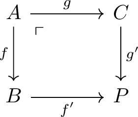
The object \(P\) is the pushout. For the diagram to “commute,” it means \(f' \circ f = g' \circ g\).
For \(T \# \mathbb{RP}^2\):
“The fundamental group of the connected sum \(M \# N\) is the pushout of the fundamental groups of the punctured surfaces along the fundamental group of the shared boundary circle.”
- Topology: The pushout of two (punctured) surfaces along a circle is their connected sum.
Example: \(A\) is the shared circle (\(S^1\)).\(B\) and \(C\) are the surfaces with holes.\(f\) and \(g\) are the inclusions.\(P\) is the connected sum.
- Algebra: The pushout of their fundamental groups is the free product with amalgamation.
Example: \(A\) is the \(\pi_1\) of shared circle (\(\mathbb{Z}\)).\(B\) and \(C\) are \(\pi_1\) of the surfaces, \(f\) and \(g\) are the induced inclusions.\(P\) is the amalgamated free product.
The Seifert-van Kampen Theorem essentially says: “The fundamental group of a pushout of spaces is the pushout of their fundamental groups.”
\(\pi_1\) is functorial, so it preserves the structure of the pushout, which is why we get the free product with amalgamation in the algebraic setting.