Week 11 Assignment: Human Neural Network Simulation

• Today, we are going to demystify the defining technology of our century: deep learning. Deep learning isn’t just about math; it is fundamentally about how information networks process raw reality to construct systems of belief.

Instructions

• Write a 1-page reflection on the simulation, and submit it to the Google Drive.
• With a partner, create a new neural network simulation that models a different historical paradigm shift (e.g., infinite different sizes of infinity, the discovery of DNA, the development of quantum mechanics, etc.). Use the same structure as the Galileo simulation, but adapt the input data and weights to fit your chosen paradigm. Submit your simulation cards and a brief explanation of your design choices to the Google Drive.
• Update you Table of Contents to include your new simulation and reflection.
• Due: Thursday, Week 12, 11:59 PM.

Thomas Kuhn and the Mechanics of ‘Loss’

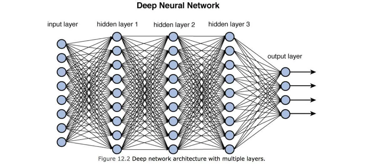
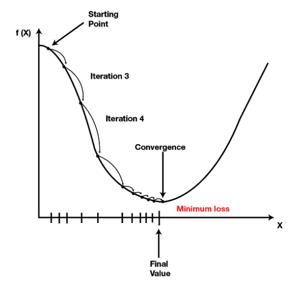
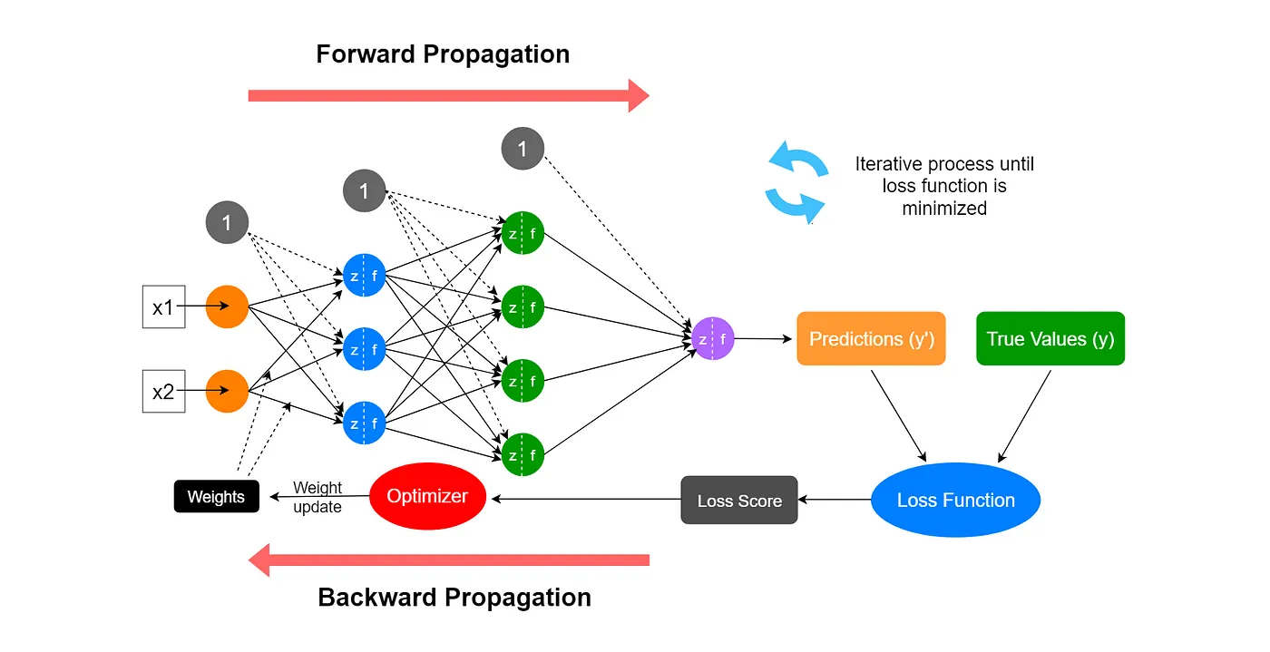
• The current dominant paradigm in AI is that of a trained neural network. But what happens when reality doesn’t match the paradigm? In deep learning, the distance between what the model predicts and what reality actually is is called the Loss. When Loss spikes, the network must adapt through Backpropagation—a retrofitting of weights. Harari might call this a self-correction mechanism. One might argue that a spike in Loss is an anomaly, and that a successful paradigm would need to be reinterpreted to accomodate for this Loss.

The Human Neural Network Simulation

Use the “Matrix” below to help you create your model of the neural network.

The Deep Learning - Kuhn - Harari Matrix

Deep Learning Term	Technical Definition	Kuhnian Paradigm Equivalent	Harari Nexus Equivalent
Neural Network	A layered architecture of artificial neurons processing data sequentially.	A community of scientists working within a shared institutional framework.	A bureaucratic network or info-web designed to generate societal order.
Input Layer	The nodes that receive raw, unweighted data points directly from the environment.	Empirical researchers observing raw phenomena (e.g., star positions, anomalies).	Low-level clerks or information gathering points in a system.
Hidden Layers	Intermediate processing stages that extract abstract features from raw inputs.	Theoretical frameworks, sub-disciplines, and peer-review filtering systems.	Mid-level bureaucratic gatekeepers who synthesize raw text into policy.
Weights & Biases	Adjustable parameters determining how heavily a node values a specific input.	The institutional prejudices, training defaults, and dogmas of ‘Normal Science’.	Institutional self-preservation rules that favor systemic stability over truth.
Loss Function	A mathematical metric measuring the error rate of a network’s prediction.	The accumulation of anomalies that cannot be explained by the dominant paradigm.	The gap between bureaucratic propaganda and structural reality.
Backpropagation	An optimization loop that adjusts weights backward based on error calculation.	The intellectual crisis and restructuring that happens during a scientific revolution.	A structural administrative reform or corrective uprising when order fails.
Overfitting	When a model memorizes its training data too perfectly but fails to generalize.	Scholastic dogmatism—solving hyper-specific puzzles while missing massive anomalies.	Rigid bureaucracies that excel at internal paperwork but collapse in a crisis.

The Paradigm Shift Neural Net

Rules

1. Information can only move sequentially from Input to Hidden Layer 1, to Hidden Layer 2, to Output.
2. The Output layer must classify the state of the world into one of two categories: Normal Science (The existing systemic framework works perfectly; anomalies are just user error) or Paradigm Shift (The core framework is broken; an intellectual revolution is mandatory).
3. Nodes must stick strictly to their specific layer functions.

How it Round Works

Before running, make each layer’s actual job explicit – not a vague “rule” or “filter,” but one specific number computed from one specific formula. The network below starts with weights inherited from the Ptolemaic paradigm: weights effectively trained by centuries of successfully saving the geocentric model from every anomaly thrown at it. Watch what those weights do to the Epoch 4 data before backpropagation touches them – that is the entire point of the exercise.

Network architecture for this round:

• 3 input nodes ->
• Hidden Layer 1 (computes one feature, “Perceived Model Strain”) ->
• Hidden Layer 2 (computes one feature, “Crisis Score”) ->
• Output (thresholds Crisis Score into Normal Science or Paradigm Shift)

PRINTABLE DATA CARD A (EPOCH 1)

• Layer Intended For: INPUT LAYER
• Role: Input nodes do no interpretation at all – they report raw values, unweighted, exactly as measured, and pass them forward unchanged.
• Environmental Data Points (reported as raw values \(x_1, x_2, x_3\)):
  • \(x_1 = 10\) – the Julian Calendar has drifted 10 full days out of alignment with the spring equinox.
  • \(x_2 = 1\) – Mars is observed in retrograde motion (a flag: 1 if observed, 0 if not).
  • \(x_3 = 40\) – the number of epicycles now required to keep orbits circular and Earth-centered.
• Input Layer Instructions: Report \(x_1, x_2, x_3\) to Hidden Layer 1. Do not interpret them – that is not this layer’s job.

PRINTABLE DATA CARD B (EPOCH 2)

• Layer Intended For: HIDDEN LAYER 1 (Feature Extractor)
• Role: Multiply each raw input by a weight and sum the result into one number: Perceived Model Strain. The weights below are not neutral – they are inherited from a paradigm already committed to geocentrism, set specifically to keep this number small.
• Current Weights (The Paradigm’s Inheritance):
  • \(w_1\) (calendar drift) \(= 0.1\) – small and dismissive: drift reads as a rounding error, not a sign of model failure.
  • \(w_2\) (retrograde motion) \(= 0.05\) – barely counted: epicycles already “explain” this, so new occurrences aren’t treated as new evidence.
  • \(w_3\) (epicycle count) \(= -0.3\) – negative. Under this paradigm, more epicycles are read as the model becoming more precise, not more strained, so a rising epicycle count actively lowers the computed strain.
• Task: Compute \(\text{Strain} = w_1 x_1 + w_2 x_2 + w_3 x_3 = (0.1)(10) + (0.05)(1) + (-0.3)(40) = 1 + 0.05 - 12 = -10.95\). Pass this single number to Hidden Layer 2.

PRINTABLE DATA CARD C (EPOCH 3)

• Layer Intended For: HIDDEN LAYER 2 (Abstract Combiner)
• Role: Take Hidden Layer 1’s Strain value and scale it by an institutional-caution weight, producing the final Crisis Score the Output layer will threshold.
• Current Weight: \(w_4\) (institutional damping) \(= 0.2\) – a strong dampening factor reflecting the Church-endorsed cosmology’s default assumption of stability.
• Task: Compute \(\text{Crisis Score} = w_4 \times \text{Strain} = 0.2 \times (-10.95) = -2.19\). Pass this number to the Output Layer.

Output Layer rule: if Crisis Score \(> 5\), output Paradigm Shift; otherwise output Normal Science. With Crisis Score \(= -2.19\), the Output Layer reports: “Normal Science. No action required.” At this point in history (pre-1543), that is in fact the defensible call – the data exists, but no rival model has yet been proposed to explain it better. No error yet, so no backpropagation yet.

Then more data arrives, and the paradigm is forced to confront a new kind of evidence.

PRINTABLE DATA CARD D (EPOCH 4 – THE INJECTION OF CRITICAL ERROR)

• Layer Intended For: INPUT LAYER (New Data Stream)
• Role: Same as Card A – report raw values, no interpretation. Note that this epoch introduces a genuinely new input, \(x_4'\), made measurable for the first time by a new instrument (the telescope) – the network has never had a weight for this kind of evidence before.
• Environmental Data Points (as raw values \(x_1', x_2', x_3', x_4'\)):
  • \(x_1' = 12\) – Gutenberg’s printing press has let mathematical tables from different cities be cross-checked; the same calendar errors show up everywhere, independently confirmed (a higher-confidence version of \(x_1\)).
  • \(x_2' = 1\) – in 1572, a new star (a supernova) appears in Cassiopeia and shines for 18 months, directly violating the axiom that the heavens are fixed and unchanging.
  • \(x_3' = 4\) – Galileo’s spyglass reveals four bodies independently orbiting Jupiter, not Earth: direct geometric evidence against “everything orbits the center.”
  • \(x_4' = 1\) – Galileo’s spyglass also reveals mountains, craters, and shadows on the Moon’s surface (a flag: 1 if observed): not geometric evidence, but metaphysical evidence – it attacks the separate claim that celestial bodies are perfect, smooth, incorruptible orbs, categorically unlike rough, imperfect Earth.
• Input Layer Instructions: Report \(x_1', x_2', x_3', x_4'\) forward, unchanged. Force the network to run a new forward pass.

Running the Old Weights on the New Data (Still Wrong)

Hidden Layer 1 has never seen \(x_4'\) before, so its weight, \(w_5\), starts at a skeptical default – the paradigm’s first instinct toward any unfamiliar instrument reading is that it’s an artifact of the equipment, not a fact about the world: \(w_5 = 0.02\) (many of Galileo’s contemporaries argued exactly this – that the telescope’s imperfect glass was producing illusions, not revealing real lunar terrain). Using the same, unchanged weights from Card B, plus this freshly initialized \(w_5\):

\[\text{Strain} = (0.1)(12) + (0.05)(1) + (-0.3)(4) + (0.02)(1) = 1.2 + 0.05 - 1.2 + 0.02 = 0.07\]

Hidden Layer 2: \(\text{Crisis Score} = 0.2 \times 0.07 = 0.014\) – nowhere near the threshold of 5.

Output Layer reports: “Normal Science.” This is now wrong – with four centuries of hindsight, Epoch 4’s evidence should classify as Paradigm Shift. The Loss is large.

Loss & Backpropagation: Correcting the Paradigm’s Weights

Trace the error backward through the network, one layer at a time:

• Output Layer: “My threshold rule is fine – Crisis Score over 5 means Shift. The number I received was just too small.”
• Hidden Layer 2: “I only scale whatever Hidden Layer 1 sends me. If Strain had come in higher, my scaled Crisis Score would have cleared the threshold easily. Hidden Layer 1, your number was too low.”
• Hidden Layer 1: “My number was too low for two separate reasons. First, \(w_3\) is negative – I’m treating Jupiter’s four orbiting moons exactly like I treated the old epicycle count, and penalizing direct geometric counter-evidence instead of registering it. Second, \(w_5\) is nearly zero – I’m dismissing the Moon’s mountains as a lens artifact instead of as real evidence against celestial perfection. Those are two different bugs: one is refusing to update on orbital evidence, the other is refusing to trust a new kind of evidence at all.”
• Professor (adjusting weights): “Network update: flip \(w_3\) from \(-0.3\) to \(+2.0\) – independent, corroborated, mechanism-breaking orbital observations must now count as strong evidence, not noise to be absorbed. Raise \(w_5\) from \(0.02\) to \(+1.0\) – a rough, cratered Moon is real evidence against the terrestrial/celestial divide, not an instrument flaw. Raise \(w_1\) from \(0.1\) to \(0.4\) – cross-city, cross-instrument agreement should matter. Raise \(w_4\) (Hidden Layer 2’s damping factor) from \(0.2\) to \(0.6\) – institutional caution should resist real evidence less than it used to.”

The Second Forward Pass (Updated Weights)

Same Epoch 4 inputs, new weights: \[\text{Strain} = (0.4)(12) + (0.05)(1) + (2.0)(4) + (1.0)(1) = 4.8 + 0.05 + 8 + 1 = 13.85\] \[\text{Crisis Score} = 0.6 \times 13.85 = 8.31\]

\(8.31 > 5\). Output Layer reports: “Paradigm Shift.”

Notice what backpropagation actually changed: not the raw observations – the Input Layer’s numbers are identical in both passes – but how much weight later layers give to each kind of observation. Notice too that the fix required correcting two distinct errors, not one: \(w_3\) was actively working against good orbital evidence, while \(w_5\) simply hadn’t learned to trust a new category of evidence yet. That is Kuhn’s argument in miniature: a revolution rarely arrives with brand-new facts nobody had seen before (Galileo’s moons and mountains were both there to observe once a telescope existed). What changes is which already-visible facts a trained community is willing to let count as evidence at all – and sometimes a community has to learn to trust a whole new kind of evidence before it can even ask whether that evidence is damning.

The Network, After Backpropagation (Part 5)

How a Node Acts Like a Neuron

Where the Analogy Breaks

• Timing: Real neurons fire discrete spikes over time and encode information in their rhythm; a node computes one number in a single step.
• Scale and wiring: A biological neuron may have thousands of synapses and many neurotransmitters; a node has a handful of numeric weights.
• Learning: Synapses change through local chemistry; networks learn by backpropagation, a global bookkeeping procedure with no known counterpart in the brain.
• Why keep the word “neural”? The analogy is inspiration, not biology: many simple units, adjustable connection strengths, and behavior that emerges from the whole network rather than from any one node. Ask the class: is that enough to call it a “neuron”?