Intro to R & Positron

Getting Started

After you have downloaded R and Positron (or maybe RStudio) open Positron (or maybe RStudio) and play around with the software. RStudio was the default IDE (Integrated Developer Environment) for R for many years.

Positron is a new IDE similar to VSCode, and is designed as an IDE for Data Science, focusing on Python & R. If you already use VSCode and Python, you should definitely try Positron.

Positron has several panes, including a Source Editor, a Workspace Browser, Plots, and a Console - each with various tabs. Learn more here.

RStudio has four main panes, the Source Editor, the Workspace Browser, the Plots, and the Console - each with various tabs. Learn more here.

Base R

Many of the features of R are available in base R, which is the default installation of R. You can use base R to do calculations, create plots, and analyze data. The base R installation is sufficient for many tasks, but there are many additional packages available that extend the functionality of R. We’ll learn about some of these packages later in the course.

R Is a Calculator

Try some calculations in the console. While you’re in the console, browse the other tabs.

3*4 - 5

[1] 7

2*4^2 - 3

[1] 29

c() and Collections

Next, the function c() stands for collection and returns a collection, or list. Make several collections, varying the kinds of elements it contains. What do you learn about the behavior?

x <- c(1:25)
x^2

 [1]   1   4   9  16  25  36  49  64  81 100 121 144 169 196 225 256 289 324 361
[20] 400 441 484 529 576 625

last_names <- c("phillips",1:5,"lebowski")

You could also use ‘list()’, whe

# Creating a list with named components
my_list <- list(name = "Alice", age = 30, scores = c(85, 92, 78))

# Accessing elements of the list using names of the components
my_list$name

[1] "Alice"

my_list$scores

[1] 85 92 78

# Accessing using the single bracket operator returns a list, while the double bracket operator returns the actual element.  For example, `my_list[1]` returns a list containing the first element, while `my_list[[1]]` returns the actual value of the first element.

my_list[1] # returns a list containing the first element (name)

$name
[1] "Alice"

my_list[3] # returns a list containing the third element (scores)

$scores
[1] 85 92 78

# Accessing elements of the list using index
my_list[[1]]  # Accessing the first element (name)

[1] "Alice"

my_list[[3]]  # Accessing the third element (scores)

[1] 85 92 78

Packages

Many data sets and much of the functionality of R exists as packages. The code below downloads the package installer pak and uses it to install the package tidyverse from CRAN. See Section 1.4.3 of the text.

The tidyverse is a collection of packages that are designed to work together and share an underlying philosophy and common APIs. The tidyverse includes packages like ggplot2, dplyr, tidyr, readr, purrr, and tibble. We’ll use these packages throughout the course. See Section 1.4.3 of the text for more information.

install.packages("pak")
library(pak)
pkg_install("tidyverse")

Loading Packages with library()

The step pkg_install("tidyverse") above merely downloads the package to your machine. It does not load it in R. To use the package you check it out from the library as follows. This loads many functions and datasets.

library(tidyverse)

── Attaching core tidyverse packages ──────────────────────── tidyverse 2.0.0 ──
✔ dplyr     1.2.1     ✔ readr     2.2.0
✔ forcats   1.0.1     ✔ stringr   1.6.0
✔ ggplot2   4.0.3     ✔ tibble    3.3.1
✔ lubridate 1.9.5     ✔ tidyr     1.3.2
✔ purrr     1.2.2     
── Conflicts ────────────────────────────────────────── tidyverse_conflicts() ──
✖ dplyr::filter() masks stats::filter()
✖ dplyr::lag()    masks stats::lag()
ℹ Use the conflicted package (<http://conflicted.r-lib.org/>) to force all conflicts to become errors

Visit section 1.4.4 for details.

Datasets

Data is everywhere - you’re encouraged to find data on your own. We will use data from a variety of sources. But to get started we’ll use some of the many datasets that are available as packages. To see a list of datasets available in base R

# see a list of data
# some are actual datasets from scientific studies
# some are synthetic data used for training algorithms, academic study, etc.
data()

This one is from a scientific study on penguins. It’s also contained in the tidyverse package.

Attaching package: 'palmerpenguins'

The following objects are masked from 'package:datasets':

    penguins, penguins_raw

Getting Help

To examine what is in this package you can use help as shown below.

help(package="palmerpenguins")

So now you see penguins is a data.frame inside this package. You can explore it in a number of ways. You can type View(penguins) to view the data in RStudio. You just type penguins, or you can look a summary of the data with summary(penguins). To see just the beginning of penguins do this:

head(penguins)

# A tibble: 6 × 8
  species island    bill_length_mm bill_depth_mm flipper_length_mm body_mass_g
  <fct>   <fct>              <dbl>         <dbl>             <int>       <int>
1 Adelie  Torgersen           39.1          18.7               181        3750
2 Adelie  Torgersen           39.5          17.4               186        3800
3 Adelie  Torgersen           40.3          18                 195        3250
4 Adelie  Torgersen           NA            NA                  NA          NA
5 Adelie  Torgersen           36.7          19.3               193        3450
6 Adelie  Torgersen           39.3          20.6               190        3650
# ℹ 2 more variables: sex <fct>, year <int>

We have data about the species Adelie and its bill length 39.1 mm, among many other things. We’ll learn how to make all kinds of graphics from datasets like this. One easy thing we can do is compare male and female bill lengths as below.

Notice the <- symbol is an assignment of the right side to the left. It is to be used to assignment, where = is used as options to functions. The <- expression can be keyed in RStudio as option - in Mac or alt - in Windows.

a <- c(1:5)

Data Frames

In the syntax below, penguins is a data frame, (like a rectangular matrix) so we can access specific entries like this:

penguins[1,2]

# A tibble: 1 × 1
  island   
  <fct>    
1 Torgersen

penguins[3,]

# A tibble: 1 × 8
  species island    bill_length_mm bill_depth_mm flipper_length_mm body_mass_g
  <fct>   <fct>              <dbl>         <dbl>             <int>       <int>
1 Adelie  Torgersen           40.3            18               195        3250
# ℹ 2 more variables: sex <fct>, year <int>

penguins[,1]

# A tibble: 344 × 1
   species
   <fct>  
 1 Adelie 
 2 Adelie 
 3 Adelie 
 4 Adelie 
 5 Adelie 
 6 Adelie 
 7 Adelie 
 8 Adelie 
 9 Adelie 
10 Adelie 
# ℹ 334 more rows

The Pipe: |>

The |> is the pipe which sends the left side (data, output of a function) to the right side (the right side is always a function, note the syntax of the right side sum().

c(1:5) |> sum()

[1] 15

The usage of the pipe may seem weird at first, but it’s ubiquitous so get used to using |>. Your code will be more readable and concise.

The pipe |> is similar to the %>% operator from the magrittr package. LLM’s often produce code using %>% but the new |> is now part of base R and is preferred. The pipe is used in many of the examples in this course. See Section 6.2 of the text for more information.

Here we use the pipe with to round a set of numbers

# make 5 random numbers
a <- 10*rnorm(5)

# two ways to round them
round(a)

[1] -8 -1 -5  2 -4

a |> round()

[1] -8 -1 -5  2 -4

# notice that the first parameter to round() is a data frame and the second
# is digits (how many decimal places to keep)

# the pipe always sends its data to the first parameter of the function
a |> round(digits = 2)

[1] -8.29 -1.14 -5.37  1.93 -3.82

# here's a list of numbers with some outliers
a <- c(-100, 0:10, 20)

# the mean
a |> mean()

[1] -1.923077

# again, the pipe sends data to the first argument of the function
# to remove the outliers from the ends we can trim
a |> mean(trim = .1)

[1] 5

Plotting with ggplot

The ggplot function is the main plotting tools we’ll use. Let’s see how the pipe |> is used in the context of ggplot(). The next two snippets are equivalent.

In the syntax of ggplot you notice that its first argument is a data frame, (this is similar to most functions) but in the code below it only accepts the aes() argument. This is because what precedes the pipe always goes into the first argument of what follows. We’ll learn this in detail later.

penguins_complete <- penguins[complete.cases(penguins),]
  ggplot(penguins_complete,aes(x = body_mass_g,y = bill_length_mm, color = sex)) +
geom_point()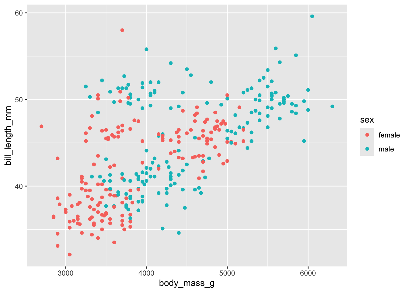

is equivalent to

penguins_complete <- penguins[complete.cases(penguins),]
penguins_complete |> 
  ggplot(aes(x = body_mass_g,y = bill_length_mm, color = sex)) +
geom_point()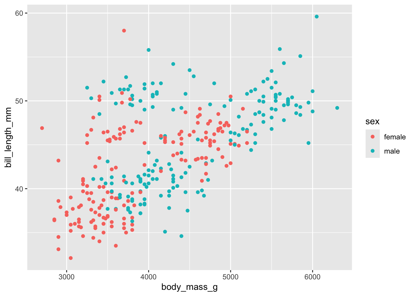

Assignment 1

The following datasets come with the tidyverse package. Choose one and create some kind of plot from it. (Datasets: midwest, USArrests, cars).

# This displays datasets that come with the tidyverse package.  Some are clean and easy to use, some are dirty by design.
data()

See https://jonpage.github.io/r-course/intro.html for inspiration. Note the syntax to refer to a specific variable penguins$bill_length_mm.

Export the plot as an image. You can submit the image in class on Wednesday.