Making Maps

Note: This is based off Sarah’s Notes

Making Maps in R

Let’s plot the global human development index (HDI). The HDI metric from the United Nations Development Program (UNDP) is a summary measure of the average achievement of a country in key dimensions of human development: a long and healthy life, being knowledgeable, and a decent standard of living (value ranges from 0 to 1, higher = better).

Load Libraries

# install.packages("maps")
# install.packages("countrycode")
library(countrycode)  # converts country names/codes between formats (needed to join our data to the map outlines)
library(dplyr)        # data wrangling (mutate, left_join, etc.)
library(stringr)      # string helpers (used if country names need cleanup)
library(ggplot2)      # plotting, including geom_polygon() for maps
library(maps)         # supplies the raw world/country outline data via map_data()

The maps package contains outlines of several continents, countries, and states (examples: world, usa, state) that have been with R for a long time. maps has its own plotting function, but we will use the map_data() function of ggplot2 to make a data frame that ggplot2 can operate on.

Create a data frame from map outlines

# map_data() turns the maps package's internal map database into a plain
# data frame of (long, lat) polygon points that ggplot2 can draw directly
world <- map_data("world")

The new world data frame has the following variables: long for longitude, lat for latitude, group tells which adjacent points to connect, order refers to the sequence by which the points should be connected, and region and subregion annotate the area surrounded by a set of points.

Make a simple world map

geom_polygon() draws maps with gray fill by default and coord_fixed() specifies the aspect ratio of the plot (every y unit is 1.3 times longer than the x unit).

world <- map_data("world")
worldplot <- ggplot() +
  # group = group tells ggplot which points belong to the same polygon
  # (a country can be made of several disconnected shapes, e.g. islands)
  geom_polygon(data = world, aes(x=long, y = lat, group = group)) + 
  # fixes the ratio between a unit of longitude and a unit of latitude so
  # the map isn't visually stretched; 1.3 is a standard approximation
  coord_fixed(1.3)
worldplot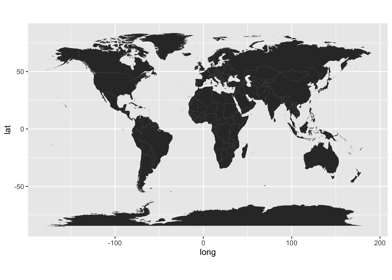

Download file from the internet directly into R

# this grabs the file and stores in your current directory
# curious where this is?  getwd() to find out where

# only download if we don't already have a local copy, so re-rendering
# the document doesn't re-fetch the file every time
if (!file.exists("hdi.data")) {
  download.file(
    url = "https://euclid.nmu.edu/~joshthom/teaching/dat309/week6/hdi.data",
    destfile = "hdi.data")
}

# this data was a tibble in R that I saved using
# write_rds(HDI,"hdi.data")
# read_rds preserves column types exactly (unlike a csv), so we use it to
# load the data back in as it was originally saved
hdi <- readr::read_rds("hdi.data")

Load the global climate event data

library(tidyverse)
# load the global climate event data: one row per climate event, including
# which country it occurred in and its economic impact
gce <- read_csv("https://euclid.nmu.edu/~joshthom/dat309/data/climate/global_climate_events_economic_impact_2020_2025.csv")

Prepare to merge data

# install.packages('countrycode')
library(countrycode)

# world, gce, and hdi all spell country names differently (e.g. "United
# States" vs "USA" vs "US"), so a direct join on name would miss matches.
# countrycode() converts every country name to the same standardized code
# (genc3c: a 3-letter government/ISO country code) so the three data sets
# can be joined reliably on that shared key ("cname").
world <- world |> mutate(cname = countrycode(
  region, 
  origin = 'country.name.en', 
  destination = 'genc3c'))

gce <- gce |> mutate(cname = countrycode(
  country, 
  origin = 'country.name.en', 
  destination = 'genc3c'))

Exercise: Understand countrycode()

Use select(), slice_sample() and pull() to extract the region from the world data. Feed this to countrycode(), keeping your eyes open to how origin and destination are used to produce a standard code for the country.

# what happened in the code above? 

Join the climate event data onto the map polygons by standardized country code, so each polygon point inherits that country’s climate impact data.

The data gce has many rows per country (one row per climate event, and some countries have 80+ events across 2020-2025), while world has many rows per country too (one row per polygon vertex).

For example, the top second country of the data begins like this

gce |> filter(country == country[2]) |> head()

# A tibble: 6 × 21
  event_id date        year month country event_type severity duration_days
  <chr>    <date>     <dbl> <dbl> <chr>   <chr>         <dbl>         <dbl>
1 EV02303  2020-01-01  2020     1 Qatar   Hurricane         1             4
2 EV00190  2020-01-23  2020     1 Qatar   Drought           4            43
3 EV02735  2020-03-13  2020     3 Qatar   Flood             4            16
4 EV00211  2020-03-21  2020     3 Qatar   Tsunami           3             1
5 EV00320  2020-03-25  2020     3 Qatar   Earthquake        2             1
6 EV02119  2020-04-17  2020     4 Qatar   Tsunami           2             1
# ℹ 13 more variables: affected_population <dbl>, deaths <dbl>, injuries <dbl>,
#   economic_impact_million_usd <dbl>, infrastructure_damage_score <dbl>,
#   response_time_hours <dbl>, international_aid_million_usd <dbl>,
#   latitude <dbl>, longitude <dbl>, total_casualties <dbl>,
#   impact_per_capita <dbl>, aid_percentage <dbl>, cname <chr>

and

a random country’s data in world looks like this

world |> filter(region == region[sample(nrow(world),1)]) |> head()

       long      lat group order    region subregion cname
1 -46.26670 60.78139   648 43088 Greenland         1   GRL
2 -46.38154 60.66031   648 43089 Greenland         1   GRL
3 -46.49634 60.68667   648 43090 Greenland         1   GRL
4 -46.55312 60.74077   648 43091 Greenland         1   GRL
5 -46.66621 60.76592   648 43092 Greenland         1   GRL
6 -46.78809 60.75840   648 43093 Greenland         1   GRL

Joining the two directly causes a many-to-many join:

• every event row for a country gets duplicated across every polygon point for that country*,

inflating the result to millions of rows and leaving impact_per_capita ambiguous (which event’s value should a given polygon point show?).

left_join(world, gce) |> nrow() |> format(big.mark = ",")

[1] "3,453,107"

We summarize gce down to one row per county first so the join becomes a clean many-to-one (many polygon points, one event summary per country).

gce_summary <- gce |>
  group_by(country, cname) |>
  summarise(impact_per_capita = mean(impact_per_capita, na.rm = TRUE), .groups = "drop")

# world goes first (left_join(world, gce_summary)) so every polygon point is
# kept even for countries with no recorded climate events -- those countries
# still need to be drawn on the map, just with a missing/NA fill value.
# Putting gce_summary first would silently drop any country not present in
# the climate event data.

world_gce <- left_join(world, gce_summary, by = "cname")

# hdi doesn't have a "cname" column yet, but it does have a "country" column
# whose name happens to match a column already present in `world` 
# 
# the mutate above isn't applied to hdi -- left_join() here falls back to
# matching on whatever columns share a name between hdi and world (likely
# none useful), so double check this join is actually matching correctly

world_hdi <- left_join(hdi, world, by = 'cname')

final plotting

gce_plot <- ggplot(data = world_gce, mapping = aes(x = long, y = lat, group = group)) + 
  coord_fixed(1.3) +
  # fill each country's polygon by its economic impact per capita, so we can
  # compare severity across countries of very different populations/sizes
  geom_polygon(aes(fill = impact_per_capita)) +
  scale_fill_viridis_c()  + 
  ggtitle("Global Events") +
  theme_minimal()

gce_plot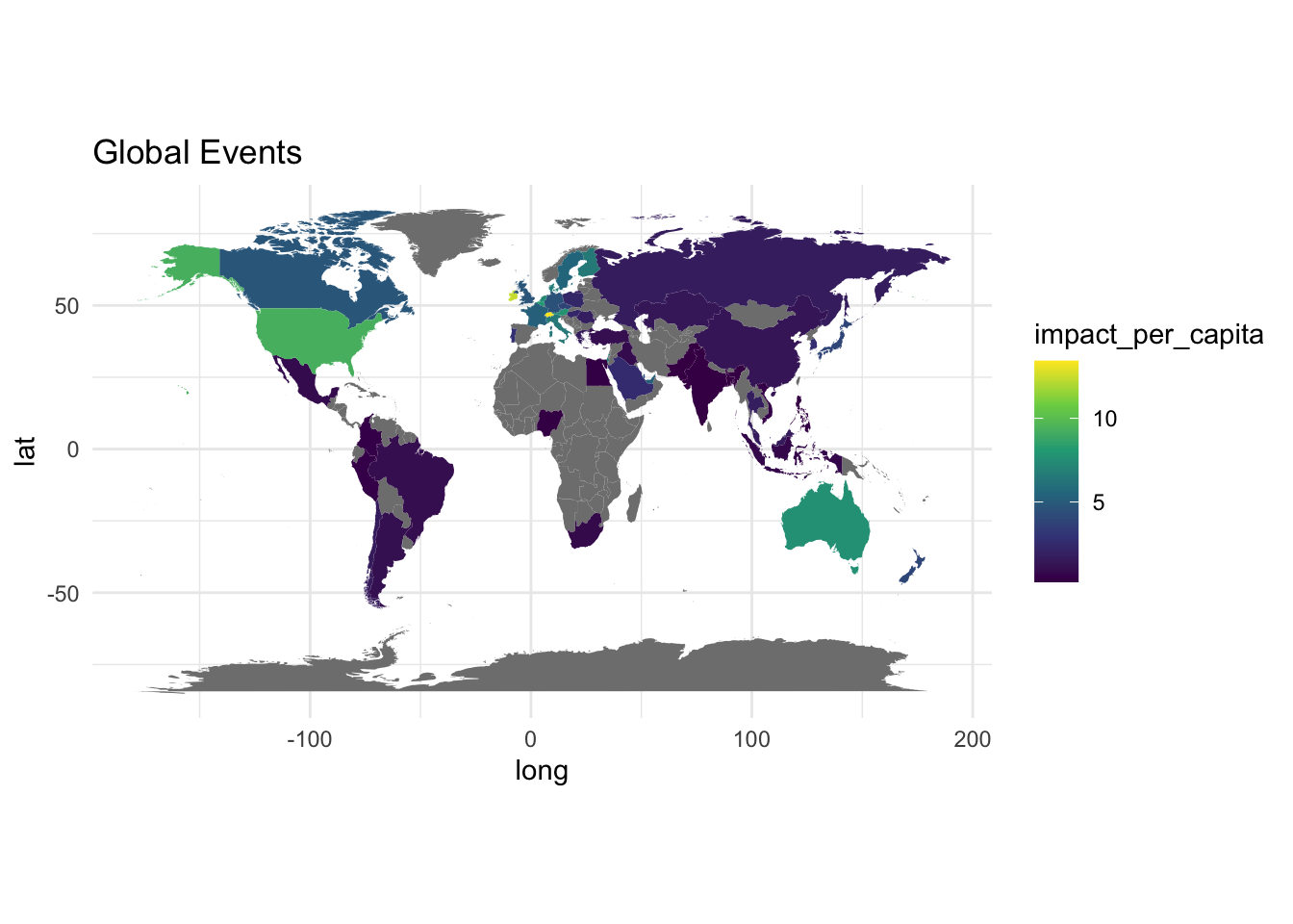

Exercise: Repeat previous plot for numeric variable

Hint: to quickly recall which variables are numeric:

gce |> select(where(is.numeric)) |> names()

 [1] "year"                          "month"                        
 [3] "severity"                      "duration_days"                
 [5] "affected_population"           "deaths"                       
 [7] "injuries"                      "economic_impact_million_usd"  
 [9] "infrastructure_damage_score"   "response_time_hours"          
[11] "international_aid_million_usd" "latitude"                     
[13] "longitude"                     "total_casualties"             
[15] "impact_per_capita"             "aid_percentage"               

HDI plot

# gni_per_capita_rank_minus_hdi_rank is a UNDP-published indicator: a
# country's rank by income (GNI per capita) minus its rank by HDI.
#   - positive value: the country ranks higher on income than on human
#     development (income isn't translating as well into health/education
#     outcomes relative to other countries)
#   - negative value: the country ranks higher on HDI than on income (it
#     achieves more human development than its income rank alone predicts)
# we map it to fill color (rather than raw hdi) because it highlights this
# relative efficiency, not just which countries are simply "richer"
gce_plot <- ggplot(data = world_hdi, 
            mapping = aes(x = long, y = lat, group = group)) + 
  coord_fixed(1.3) +
  geom_polygon(aes(fill = gni_per_capita_rank_minus_hdi_rank)) +
  # diverging palette centered near zero: red/blue show which side of the
  # income-vs-development tradeoff each country falls on
  scale_fill_distiller(palette ="RdBu", direction = -1) + # or direction=1
  ggtitle("Global Events") +
  theme_minimal()

gce_plot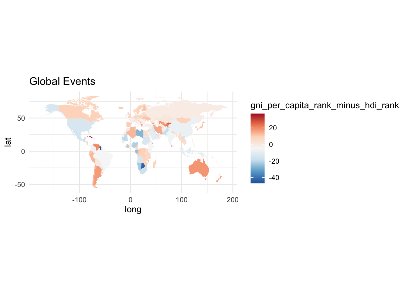

Exercise

Create a map that includes an animation.